7.12 The F Ratio
PRE alone, therefore, is not a sufficient guide in our quest to reduce error. Yes, it tells us whether we are reducing error. But it does not take into account the cost of that reduction. The F ratio provides a solution to this problem, giving us an indicator of the amount of error reduced by a model that adjusts for the number of parameters it takes to realize the reduction in error.
Let’s go back to our analysis of variance table (reprinted below). We want to take a moment to appreciate why the ANOVA tables (printed by the function supernova()) are called ANalysis Of VAriance tables. One definition of “analyze” is to break up into parts. Analysis of variance is when we break apart, or partition, variation.
We have already discussed how we analyze the SS column and break it into parts. Let’s now look at the next three columns in the table: df, MS, and F. Just a note: df stands for degrees of freedom, MS stands for Mean Square, and F, well, that stands for the F ratio.
We will start by looking at the last row of the supernova table for the Height2Group model.
Analysis of Variance Table (Type III SS)
Model: Thumb ~ Height2Group

                               SS  df      MS      F    PRE     p
----- --------------- | --------- --- ------- ------ ------ -----
Model (error reduced) |   830.880   1 830.880 11.656 0.0699 .0008
Error (from model)    | 11049.331 155  71.286
----- --------------- | --------- --- ------- ------ ------ -----
Total (empty model)   | 11880.211 156  76.155
Degrees of Freedom
We already have discussed the column labeled SS. The next column, labeled df, shows us degrees of freedom. For our Fingers data set, which has a sample of 157 students, degrees of freedom for the empty model is 156, which is \(n-1\).
Technically, the degrees of freedom of an estimate is the number of independent pieces of information that went into calculating the estimate. We find it’s helpful to think about degrees of freedom as a budget. The more data (represented by \(n\)) you have, the more degrees of freedom you have. Whenever you estimate a parameter, you spend (or lose) a degree of freedom because a parameter will limit the freedom of those data points.
What does it mean to “limit the freedom of data points”? Let’s say we have a distribution with three scores and the mean is 5. If we know the mean is 5, do we really have three data points that could be any value? Not really. If we know the mean is 5, then if we know any two of the three numbers, we can figure out the third. So even though two of the data points can be any value, the third is restricted because the mean has to be 5. So, we say there are only two (or \(n-1\)) degrees of freedom.
In the ANOVA table the bottom row is labeled “Total (empty model).” The empty model consists of a single parameter estimate, \(b_0\), which costs us one degree of freedom. Our initial df budget was 157 because we started off with 157 data points, \(n\). Given that we spent one, the degrees of freedom is now 156, \(n - 1\).
Mean Square (MS)
The third column is labeled MS, which stands for mean square error. MS is calculated by dividing SS Total (11880.211) by degrees of freedom (156), which results in an MS of 76.155.
You may recall from the previous chapter that SS divided by df is the formula for variance. You can think of MS Total as the average squared error from the mean. Variance and MS are just two names for the same thing.
Try it out. We’ve written the code to calculate the variance of Thumb length using the function var(). Use R as a calculator and try taking the sum of squares for the empty model and dividing by the degrees of freedom. You should get the same result for both methods.
require(coursekata)

Fingers <- Fingers %>% mutate(
    Height2Group = factor(ntile(Height, 2), 1:2, c("short", "tall")),
    Height3Group = factor(ntile(Height, 3), 1:3, c("short", "medium", "tall"))
)

Height2Group_model <- lm(Thumb ~ Height2Group, data = Fingers)

Height3Group_model <- lm(Thumb ~ Height3Group, data = Fingers)

empty_model <- lm(Thumb ~ NULL, data = Fingers)
# this calculates the variance of Thumb
# don't remove this line
var(Fingers$Thumb)

# try taking the SS from the empty model and dividing it by df (you can get these numbers from the supernova table; the model is loaded for you as Height2Group_model)
11880.21 / 156
ex() %>% check_output("(76\\.15.*){2}", missing_msg = "We are testing against values that start 76.15")
success_msg("G-R-eat job!")[1] 76.1552
[1] 76.1552Partitioning Degrees of Freedom
Now look again at the degrees of freedom (df) column in the table. Just as SS can be partitioned into SS Error and SS Model, df for model and df for error add up to degrees of freedom total. Let’s see why the degrees of freedom are partitioned as they are between model and error.
                               SS  df      MS      F    PRE     p
----- --------------- | --------- --- ------- ------ ------ -----
Model (error reduced) |   830.880   1 830.880 11.656 0.0699 .0008
Error (from model)    | 11049.331 155  71.286
----- --------------- | --------- --- ------- ------ ------ -----
Total (empty model)   | 11880.211 156  76.155
Remember the idea that degrees of freedom is like a budget? The more data (represented by \(n\)) you have, the more degrees of freedom you have. Whenever you estimate a parameter, you spend a degree of freedom. More complex models cost more degrees of freedom because they estimate more parameters.
Let’s think about our data on thumb lengths in the Fingers data frame. We start with \(n = 157\) thumbs, but as soon as we estimate the empty model we have already used one degree of freedom, leaving us with \(n-1\) (or 156) degrees of freedom. (The parameter we’ve estimated for the empty model is the Grand Mean). As we add explanatory variables (and new parameters) to the model, we will be “spending” from our remaining 156 degrees of freedom.
Whereas we estimate one parameter for the empty model, we estimate two for the two-group model (Height2Group_model): the mean of group one, and the increment to get to group two. This is reflected in the table by a Model df (degrees of freedom) of 1, representing the one additional degree of freedom used beyond the one used in the empty model.
If we look at the row labeled “Model (error reduced)” in the table, we can see what we “bought” for the price of one additional degree of freedom beyond the empty model: a reduction in SS of 830.88 compared with the empty model.
                               SS  df      MS      F    PRE     p
----- --------------- | --------- --- ------- ------ ------ -----
Model (error reduced) |   830.880   1 830.880 11.656 0.0699 .0008
Error (from model)    | 11049.331 155  71.286
----- --------------- | --------- --- ------- ------ ------ -----
Total (empty model)   | 11880.211 156  76.155
The empty model costs us one df (leaving us with a Total df of 156). If we spend just one more df, we can fit the two-group model, bringing the balance remaining in our df budget down to 155, which is called df Error. A general rule of thumb (no pun intended) is this: every time you add a parameter to a model you “spend” one degree of freedom.
Varieties of MS
If you take the SS and divide by the degrees of freedom you end up with Mean Square (or MS). Because we have different SS on each row of the supernova table, each with its own degrees of freedom, we have a different kind of MS (also called variance) on each row.
                               SS  df      MS      F    PRE     p
----- --------------- | --------- --- ------- ------ ------ -----
Model (error reduced) |   830.880   1 830.880 11.656 0.0699 .0008
Error (from model)    | 11049.331 155  71.286
----- --------------- | --------- --- ------- ------ ------ -----
Total (empty model)   | 11880.211 156  76.155
The last row of the table, labeled “Total (empty model)”, shows us MS Total, which can be written like this: \({MS}_{Total}\). This is calculated by dividing SS Total by the degrees of freedom for the empty model (156):
\[{MS}_{Total} = {SS}_{Total}/{df}_{Total}\]
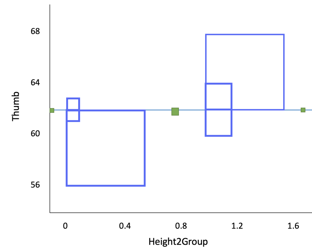
This results in an MS Total of 76.16, which is the variance of the outcome variable. The meaning of this number can be understood by reference to the blue squares in the figure below, which, for purposes of illustration, shows the TinyFingers data set. Each blue square represents the squared deviation of a single data point from the empty model prediction (or Grand Mean). MS Total is roughly the average area of these blue squares.
MS Model and MS Error are calculated in a similar way as MS Total, working across the rows of the table:
\[{MS}_{Model} = {SS}_{Model}/{df}_{Model}\]
\[{MS}_{Error} = {SS}_{Error}/{df}_{Error}\]
The three different types of MS are all variances. One is based on the deviations of the model predictions from the Grand Mean, which is the prediction of the empty model (MS Model); another on the deviations of individual scores from the model predictions (MS Error); and the third on the deviations of individual scores from the empty model prediction (MS Total).
MS Model represents the reduction in error achieved by the model (measured in SS) per degree of freedom spent beyond the empty model. MS Error tells us how much variation is left over from the complex model, again per degree of freedom left in your budget after fitting the model.
The F Ratio
Now let’s get to the F ratio. In our table, we have produced two different estimates of variance under the Height2Group model: MS Model and MS Error.
                               SS  df      MS      F    PRE     p
----- --------------- | --------- --- ------- ------ ------ -----
Model (error reduced) |   830.880   1 830.880 11.656 0.0699 .0008
Error (from model)    | 11049.331 155  71.286
----- --------------- | --------- --- ------- ------ ------ -----
Total (empty model)   | 11880.211 156  76.155
MS Model tells us what the variance would be if every student were assumed to have the thumb length predicted by the Height2Group model; MS Error tells us what the leftover variance would be after subtracting out the model. The F ratio is calculated as the MS Model divided by the MS Error:
\[F = \frac{M\!S_{Model}}{M\!S_{Error}} = \frac{S\!S_{Model}/d\!f_{Model}}{S\!S_{Error}/d\!f_{Error}}\]
This ratio turns out to be a very useful statistic. If there were no effect of Height2Group on thumb length we would expect the variance estimated using the group means to be approximately the same as the variance within the groups, resulting in an F ratio of approximately 1. But if the variation across groups is more than the variation within groups, the F ratio would rise above 1. A larger F ratio means a stronger effect of our model.
Just like variance provided us with a way to account for sample size when using SS to measure error from our model, the F ratio provides a way to take degrees of freedom into account when judging the fit of a model. The F ratio gives us a sense of whether the degrees of freedom that we spent in order to make our model more complicated were “worth it”.
Another Way of Thinking About the F Ratio
There is another way of thinking about F that makes clearer the relationship between F and PRE. It is represented by this alternative formula for F:
\[F = \frac{PRE/{df}_{model}}{(1-{PRE})/{df}_{error}}\]
This formula produces the same result as the formula for F presented in the previous section, but makes it easier to think about the relation between PRE and F.
The numerator of this formula gives us an indicator of how much PRE we have achieved in our model per degree of freedom spent (i.e., number of parameters estimated beyond the empty model). In the case of our two-group Height2Group model, it would simply be PRE divided by 1 because we used only one additional degree of freedom.
The denominator tells us how much error could be reduced (\(1-{PRE}\)) per degree of freedom if we were to put all still-unused degrees of freedom (\({df}_{error}\)) into the model. In other words, it tells us what the PRE would be, on average, if we just randomly picked a parameter to estimate instead of the one that we picked for our model.
The F ratio, thought of this way, compares the amount of PRE achieved by the particular parameters we included in our model (per parameter) to the average amount of remaining PRE that could have been achieved by adding all the possible remaining parameters into the model.
Or put another way, the F ratio answers this question: How many times bigger is the PRE obtained by our best fitting model (per degree of freedom spent) compared to the average PRE that could have been obtained (again, per degree of freedom) by spending all of the possible remaining degrees of freedom?