8.3 Fitting a Regression Model
Using lm() to Fit the Height Model to TinyFingers
Now you can begin to see the power you’ve been granted by the General Linear Model. Fitting—or estimating the parameters—of the regression model, is accomplished the same way as estimating the parameters of the grouping model. It’s all done using the lm() function in R.
The lm() function is smart enough to know that if the explanatory variable is quantitative, it should estimate the regression model. If the explanatory variable is categorical (e.g., defined as a factor in R), lm() will fit a group model.
Modify the code below to fit the regression model using Height as the explanatory variable to predict Thumb length in the TinyFingers data.
require(coursekata)

TinyFingers <- data.frame(
    Sex = as.factor(rep(c("female", "male"), each = 3)),
    Thumb = c(56, 60, 61, 63, 64, 68),
    Height = c(62, 66, 67, 63, 68, 71)
)  %>% mutate(
    Height2Group = recode(ntile(Height, 2), '1' = "1-Short", '2' = "2-Tall"),
    Height3Group = recode(ntile(Height, 2), '1' = "1-Short", '2' = "2-Medium", '3' = "3-Tall")
)
# modify this to fit Thumb as a function of Height
Tiny_Height_model <- lm()

# this prints the best-fitting estimates
Tiny_Height_model
Tiny_Height_model <- lm(Thumb ~ Height, data = TinyFingers)
Tiny_Height_model
ex() %>% {
    check_object(., "Tiny_Height_model") %>% check_equal()
    check_output_expr(., "print(Tiny_Height_model)")
}Call:
lm(formula = Thumb ~ Height, data = TinyFingers)
Coefficients:
(Intercept) Height
-3.1611 0.9848Fitting a Regression Model By Accident When You Don’t Want One
Although R is pretty smart about knowing which model to fit, it won’t always do the right thing. If you code the grouping variable with the character strings “short” and “tall,” R will make the right decision because it knows the variable must be categorical. But if you code the same grouping variable as 1 and 2, and you forget to make it a factor, R may get confused and fit the model as though the explanatory variable is quantitative.
For example, we’ve added a new variable to our TinyFingers data called GroupNum. Here is what the data look like.
  Thumb Height Height2Group GroupNum
1    56     62        Short        1
2    60     66        Short        1
3    61     67         Tall        2
4    63     63        Short        1
5    64     68         Tall        2
6    68     71         Tall        2
If you take a look at the variables Height2Group and GroupNum, they have the same information. Students 1, 2, and 4 are in one group and students 3, 5, and 6 are in another group. If we fit a model with Height2Group (and called it the Height2Group_model) or GroupNum (and called it the GroupNum_model), we would expect the same estimates. Let’s try it.
require(coursekata)

TinyFingers <- data.frame(
    Sex = as.factor(rep(c("female", "male"), each = 3)),
    Thumb = c(56, 60, 61, 63, 64, 68),
    Height = c(62, 66, 67, 63, 68, 71)
)  %>% mutate(
    Height2Group = recode(ntile(Height, 2), '1' = "1-Short", '2' = "2-Tall"),
    Height3Group = recode(ntile(Height, 2), '1' = "1-Short", '2' = "2-Medium", '3' = "3-Tall"),
    GroupNum = ntile(Height, 2)
)
# fit a model of Thumb length based on Height2Group
Height2Group_model <- lm()

# fit a model of Thumb length based on GroupNum
GroupNum_model <- lm()

# this prints the parameter estimates from the two models
Height2Group_model
GroupNum_model
Height2Group_model <- lm(Thumb ~ Height2Group, data = TinyFingers)
GroupNum_model <- lm(Thumb ~ GroupNum, data = TinyFingers)
Height2Group_model
GroupNum_model
ex() %>% {
    check_object(., "Height2Group_model") %>% check_equal()
    check_object(., "GroupNum_model") %>% check_equal()
    check_output_expr(., "Height2Group_model
GroupNum_model")
}Call:
lm(formula = Thumb ~ Height2Group, data = TinyFingers)
Coefficients:
(Intercept) Height2GroupTall
59.667 4.667
Call:
lm(formula = Thumb ~ GroupNum, data = TinyFingers)

Coefficients:
(Intercept)     GroupNum
55.000 4.667Because Height2Group is a factor (i.e., a categorical variable), lm() fits a group model. But for GroupNum, lm() thinks the 1 or 2 coding refers to a quantitative variable. Because we did not tell R to treat GroupNum as a factor, it fits a regression line instead of a two-group model. If it does that, the meaning of the estimates will not be what you expect for the group model.
The \(b_{1}\) estimate will be the same as in the two-group model; because it represents the slope of the regression line, it will tell you the increment in thumb length between people coded as 2 versus those coded as 1. But the \(b_{0}\) estimate will be different in the regression model, where it represents the y-intercept of the regression line, or the predicted thumb length when \(X_{i}\) equals 0. This makes no sense, however, when there are only two groups and they are coded 1 and 2. This is an accidental regression model.
Try it here by recoding GroupNum as 0 and 1. See if the results fit your expectations.
require(coursekata)

TinyFingers <- data.frame(
    Sex = as.factor(rep(c("female", "male"), each = 3)),
    Thumb = c(56, 60, 61, 63, 64, 68),
    Height = c(62, 66, 67, 63, 68, 71)
)  %>% mutate(
    Height2Group = recode(ntile(Height, 2), '1' = "1-Short", '2' = "2-Tall"),
    Height3Group = recode(ntile(Height, 2), '1' = "1-Short", '2' = "2-Medium", '3' = "3-Tall"),
    GroupNum = ntile(Height, 2)
)
Height2Group.model <- lm(Thumb ~ Height2Group, data = TinyFingers)
# recode GroupNum from 1 and 2 to 0 and 1
# save it to a new variable Group01 so that nothing is overwritten
TinyFingers$Group01 <- recode()

# This will fit an "accidental" regression model
lm(Thumb ~ Group01, data = TinyFingers)
# recode GroupNum from 1 and 2 to 0 and 1
# save it to a new variable Group01 so that nothing is overwritten
TinyFingers$Group01 <- recode(TinyFingers$GroupNum, "1" = 0, "2" = 1)

# This will fit an "accidental" regression model
lm(Thumb ~ Group01, data = TinyFingers)
ex() %>% {
    check_object(., "TinyFingers") %>% check_column("Group01")  %>% check_equal()
    check_output_expr(., "lm(Thumb ~ Group01, data = TinyFingers)")
}Fitting the Height Model to the Full Fingers Data Set
Now that you have looked in detail at the tiny set of data, fit the height model to the full Fingers data frame, and save the model in an R object called Height_model.
require(coursekata)

Fingers <- filter(Fingers, Thumb >= 33 & Thumb <= 100)
# modify this to fit the Height model of Thumb for the Fingers data
Height_model <-

# this prints best estimates
Height_model
Height_model <- lm(Thumb ~ Height, data = Fingers)
Height_model
ex() %>% {
    check_object(., "Height_model") %>% check_equal()
    check_output_expr(., "Height_model")
}Call:
lm(formula = Thumb ~ Height, data = Fingers)
Coefficients:
(Intercept) Height
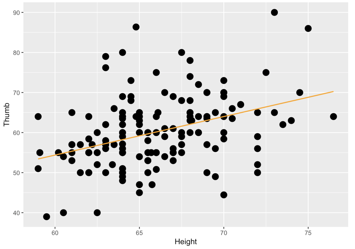
-3.3295 0.9619Here is the code to make a scatterplot to show the relationship between Height (on the x-axis) and Thumb (on the y-axis) for TinyFingers. Note that the code also overlays the best-fitting regression line on the scatterplot. Edit the code to make this scatterplot for the full Fingers data set.
require(coursekata)

Fingers <- filter(Fingers, Thumb >= 33 & Thumb <= 100)
# edit this code to create a scatterplot for the FULL Fingers data
gf_point(Thumb ~ Height, data = TinyFingers, size = 4) %>%
    gf_lm(color = "orange")
gf_point(Thumb ~ Height, data = Fingers, size = 4) %>%
    gf_lm(color = "orange")
ex() %>% check_function("gf_point") %>% check_arg("data") %>% check_equal()
success_msg("You R an R wizard!")
Simulating \(b_{1}\) Under the Empty Model (Revisited)
In Chapter 7, we spent some time revisiting the tipping study. We modeled the data using a two-group model, and found tables that got a smiley face on the check tipped $6 more, on average, than those that didn’t.
Although there was a $6 advantage of smiley face in our data, what we really want to know is: what is the advantage, if any, in the Data Generating Process? Could the $6 advantage we observed have been generated randomly by a DGP in which there is no advantage (i.e., a model in which \(\beta_{1}=0\)?
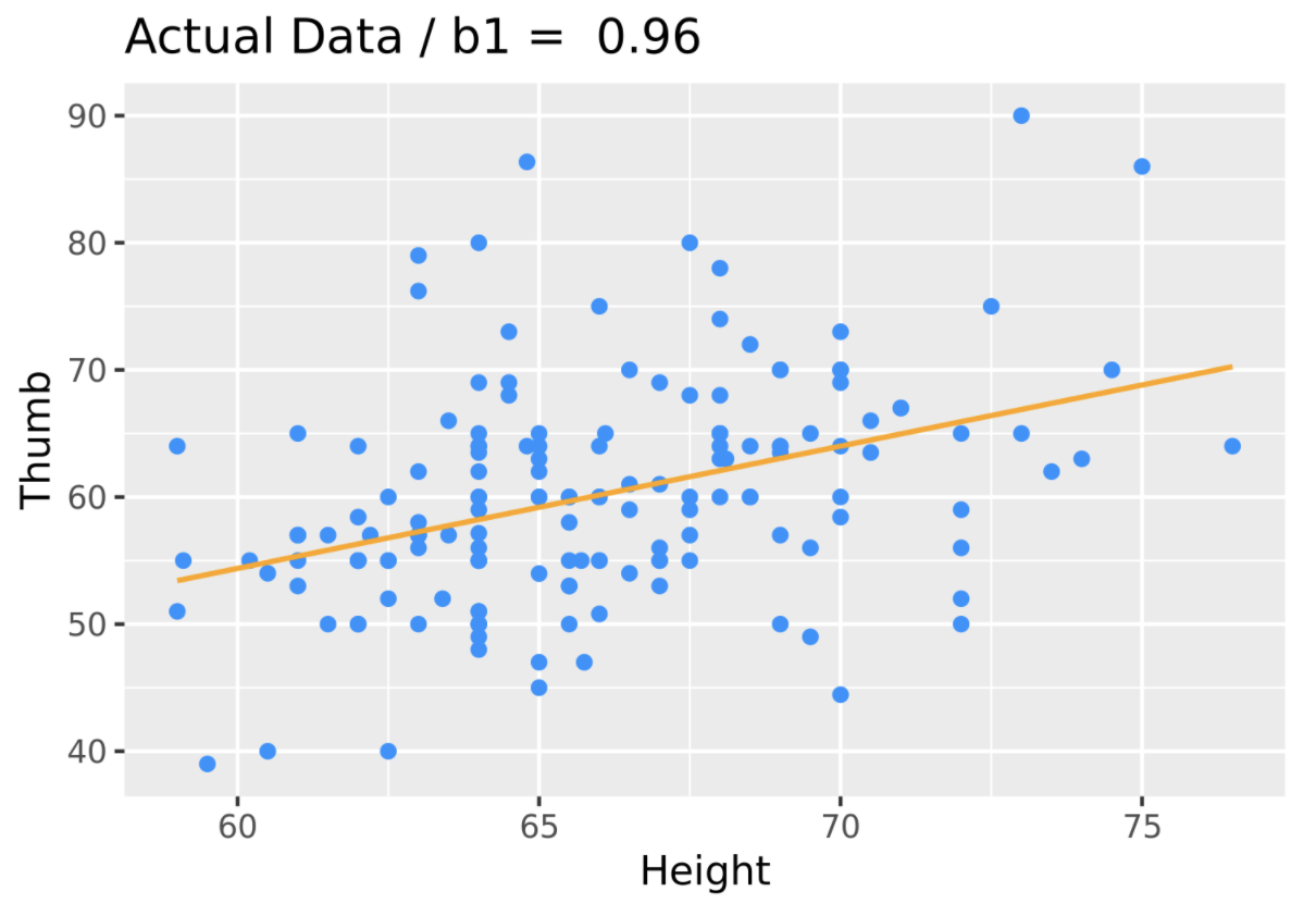
It turns out we can ask the same question with a regression model, in which \(\beta_{1}\) is a slope instead of a group difference. When we fit a regression model, regressing Height on Thumb, our best fitting estimate of the true slope (\(\beta_{1}\)) was 0.96. But could this relationship in our data have been generated by a DGP in which \(\beta_{1}=0\)?
We can ask this question by using the shuffle() function to simulate a DGP in which the empty model is true. This time, instead of shuffling which condition tables are in we will shuffle one of the two variables in our model, Thumb or Height. In this case, it doesn’t really matter which one we shuffle; we could even shuffle both. In general, it’s best to shuffle the outcome variable.
By randomly shuffling one of these variables we are simulating a DGP in which there is absolutely no relationship between the two variables, and in which any apparent relationship that appears could only be due to randomness, and not a real relationship in the DGP. If the relationship in our data was a real one, shuffling breaks it, and it isn’t real any more!
Let’s see how this works graphically. The code produces a scatterplot of Thumb by Height along with the best fitting regression line. We added in a line of code (gf_labs()) that prints the slope estimate as a title at the top of the graph.
sample_b1 <- b1(Thumb ~ Height, data = Fingers)

gf_point(Thumb ~ Height, data = Fingers, color = "dodgerblue") %>%
   gf_lm(color = "orange") %>%
   gf_labs(title = paste("Actual Data: b1 = ", round(sample_b1, digits = 2)))
Now let’s see what happens if we shuffle the variable Height before we produce the graph and best-fitting line. We accomplish this by simply adding a line of code right before the gf_point() that creates a new variable named ShuffThumb, and then plotting ShuffThumb by Height.
Fingers$ShuffThumb <- shuffle(Fingers$Thumb)
shuffled_b1 <- b1(ShuffThumb ~ Height, data = Fingers)

gf_point(ShuffThumb ~ Height, data = Fingers, color = "dodgerblue") %>%
   gf_lm(color = "orange") %>%
   gf_labs(title = paste("Shuffled Data: b1 = ", round(shuffled_b1, digits = 2)))
We’ve added the shuffle code into the window below, and also changed the gf_labs() code to title the graph Shuffled Data instead of Actual Data. Go ahead and run the code and see if it does what you thought it would. Run it a few times, and see how it changes.
require(coursekata)
Fingers$ShuffThumb <- shuffle(Fingers$Thumb)
shuffled_b1 <- b1(ShuffThumb ~ Height, data = Fingers)

gf_point(ShuffThumb ~ Height, data = Fingers, color = "dodgerblue") %>%
   gf_lm(color = "orange") %>%
   gf_labs(title = paste("Shuffled Data: b1 = ", round(shuffled_b1, digits = 2)))
# no solution; commenting for submit button
ex() %>% check_error()
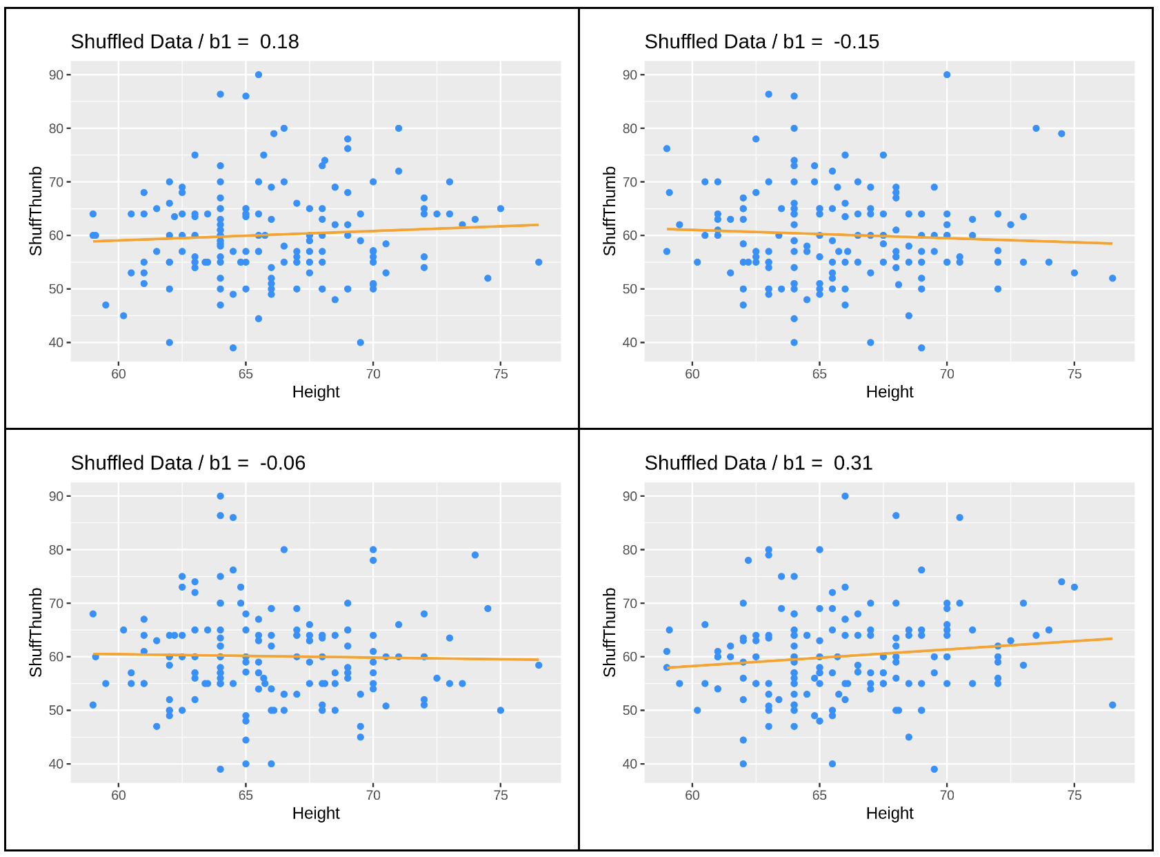
You can see that the \(b_{1}\)s vary each time you run the code, but they seem to be clustered around 0, a little negative or a little positive. This makes sense because we know that the true \(\beta_{1}\) in this case is 0. And how do we know that? Because we know that any relationship between Thumb and Height is purely random due to the fact that we shuffled one of the variables randomly.
Instead of producing a graph, we can also just produce a \(b_{1}\) directly by using the b1() function together with shuffle():
b1(shuffle(Thumb) ~ Height, data = Fingers)Use the code window below to do this 10 times and produce a list of 10 \(b_{1}\)s.
require(coursekata)
set.seed(42)
# use do() to create 10 shuffled b1s
# use do() to create 10 shuffled b1s
do(10) * b1(shuffle(Thumb) ~ Height, data = Fingers)
ex() %>% {
    check_function(., 'do') %>%
        check_arg('object') %>% check_equal()
    check_function(., 'b1') %>% {
        check_arg(., 'object') %>% check_equal(eval = FALSE)
        check_arg(., 'data') %>% check_equal()
    }
}Here are the 10 \(b_{1}\)s we generated (your list would differ, of course, because each one is based on a new random shuffle):
             b1
1   0.059185509
2  -0.013442382
3   0.027153003
4  -0.008801673
5   0.007565065
6   0.219193990
7  -0.132471001
8   0.035662413
9  -0.157540915
10 -0.035323177
As we did previously for the tipping study, we can use this list of \(b_{1}\)s generated by random shuffles of the data to help us put our observed \(b_{1}\) of 0.96 in context. Here we arranged these \(b_1\)s in order (smallest to largest) to make it easier to compare them to our sample \(b_1\).
             b1
1  -0.157540915
2  -0.132471001
3  -0.035323177
4  -0.013442382
5  -0.008801673
6   0.007565065
7   0.027153003
8   0.035662413
9   0.059185509
10  0.219193990
As you can see, these randomly generated \(b_{1}\)s cluster around 0 – roughly half are negative and half are positive. This makes sense given that their parent (\(\beta_1\)) was equal to 0. None of them come anywhere close to being as high as our sample estimate of 0.96.