9.7 Hypothesis Testing for Regression Models
We have gone through the logic of hypothesis testing for group models. We have used shuffle() to create a sampling distribution assuming that \(\beta_1=0\), and then used the sampling distribution to calculate the probability of our sample \(b_1\) or one more extreme having come from the empty model.
Now let’s apply the same ideas to regression models. As you will see, the strategy is exactly the same. We still want to create a sampling distribution of \(b_1\)s, though this time the \(b_1\) will represent a slope, not a group difference. Let’s see how this works by adding a new variable to the tipping experiment data frame.
Tips = Size of Check + Other Stuff
Often, when deciding how much to tip in the United States, people tip some percentage of their check, the total amount they spent. If they spent a lot at dinner, they would tip more, and if they spent less they would tip less.
We have added a new variable to the TipExperiment data frame: Check. Check is the total amount of the check for each table.
  TableID Tip Condition    Check
1       1  39   Control 194.0299
2       2  36   Control 352.9412
3       3  34   Control 382.0225
4       4  34   Control 204.8193
5       5  33   Control 146.6667
6       6  31   Control 254.0984
We created a scatterplot to explore the hypothesis that Check might explain some of the variation in Tip.
gf_point(Tip ~ Check, data = TipExperiment)Modeling Variation in Tips as a Function of Total Check
Use the code window below to fit a regression model in which Check is used to explain Tip.
require(coursekata)

# Simulate Check
set.seed(22)
x <- round(rnorm(1000, mean=15, sd=10), digits=1)
y <- x[x > 5 & x < 30]
TipPct <- sample(y, 44)
TipExperiment$Check <- (TipExperiment$Tip / TipPct) * 100
# fit a regression model in which Check is used to explain Tip
# fit a regression model in which Check is used to explain Tip
lm(Tip ~ Check, data = TipExperiment)
ex() %>%
    check_function("lm") %>%
    check_result() %>%
check_equal()Call:
lm(formula = Tip ~ Check, data = TipExperiment)
Coefficients:
(Intercept) Check
18.74805 0.05074A .05 increase in tip for every additional dollar spent on the meal does not seem like very much. In fact, it seems pretty close to 0. Is it possible that this \(b_1\) could have been generated by a DGP in which there is no effect of check, that is, a DGP where \(\beta_1=0\)? Or, can we reject the empty model in favor of one in which Check does effect Tip?
Evaluating the Empty Model of the DGP
Just as we did with the Condition model, we can use shuffle() to simulate the case where the empty model is true (i.e., where the true value of the slope in the DGP is 0), create a sampling distribution of \(b_1\)s by shuffling Tip, and then use the sampling distribution to calculate the likelihood of a \(b_1\) as extreme as .05 being generated by the empty model.
In the code block below we have written code to create a scatterplot of the data. Add shuffle() around the outcome (Tip) to generate a sample of shuffled data from the empty model of the DGP and plot the data with the best fitting regression line. Run it a few times just to see what kinds of slopes (\(b_1\)s) are generated by this DGP.
require(coursekata)

# Simulate Check
set.seed(22)
x <- round(rnorm(1000, mean=15, sd=10), digits=1)
y <- x[x > 5 & x < 30]
TipPct <- sample(y, 44)
TipExperiment$Check <- (TipExperiment$Tip / TipPct) * 100
# modify this to shuffle the data
gf_point(Tip ~ Check, data = TipExperiment) %>%
  gf_lm()
gf_point(shuffle(Tip) ~ Check, data = TipExperiment) %>%
  gf_lm()
ex() %>%
  check_or(
    check_function(., "gf_lm") %>%
      check_result() %>%
      check_equal(),
    override_solution_code(., "gf_point(Tip ~ shuffle(Check), data = TipExperiment) %>% gf_lm()") %>%
      check_function("gf_lm") %>%
      check_result() %>%
      check_equal()
  )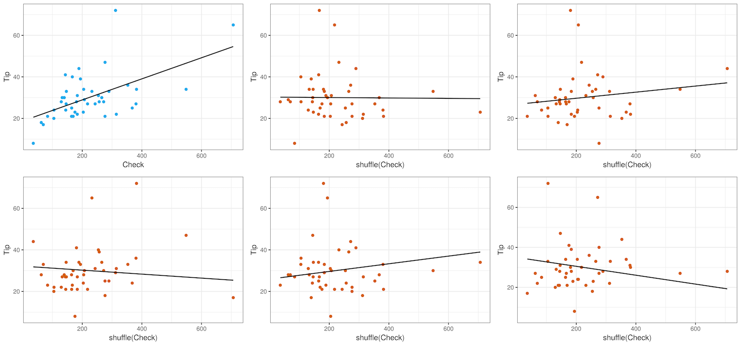
The actual data from the tipping study is shown in blue (the panel in the upper left) along with the best fitting regression line (the slope is .05). The 5 other plots (with red dots) are shuffled data, along with their best fitting regression lines.
From the shuffled data, we saw that many of the regression lines are flatter than the line for the actual data. This makes sense given that we are simulating a DGP in which \(\beta_1=0\); we would expect many of the \(b_1\)s to be close to 0. Now let’s generate a sampling distribution of \(b_1\)s using the b1() function.
Complete the first line of code below to generate a sampling distribution of 1000 \(b_1\)s (sdob1) from the Check model fit to shuffled data. We have added some additional code to generate a histogram of the sampling distribution of \(b_1\)s and represent the sample \(b_1\) as a black dot.
require(coursekata)

# Simulate Check
set.seed(22)
x <- round(rnorm(1000, mean=15, sd=10), digits=1)
y <- x[x > 5 & x < 30]
TipPct <- sample(y, 44)
TipExperiment$Check <- (TipExperiment$Tip / TipPct) * 100

sample_b1 <- b1(Tip ~ Check, data = TipExperiment)
# generate a sampling distribution of 1000 b1s from the shuffled data
sdob1 <- do() * b1()

# histogram of the 1000 b1s
gf_histogram(~ b1, data = sdob1, fill = ~middle(b1, .95), bins = 100, show.legend = FALSE) %>%
  gf_point(x = sample_b1, y = 0, show.legend = FALSE)
# generate a sampling distribution of 1000 b1s from the shuffled data
sdob1 <- do(1000) * b1(shuffle(Tip) ~ Check, data = TipExperiment)

# histogram of the 1000 b1s
gf_histogram(~ b1, data = sdob1, fill = ~middle(b1, .95), bins = 100, show.legend = FALSE) %>%
  gf_point(x = sample_b1, y = 0, show.legend = FALSE)
ex() %>% check_or(.,
  check_function(., 'b1') %>% {
    check_arg(., 1) %>% check_equal(eval = FALSE)
    check_arg(., 2) %>% check_equal()
  },
  override_solution_code(., "sdob1 <- do(1000) * b1(Tip ~ shuffle(Check), data = TipExperiment)") %>%
    check_function(., 'b1') %>% {
      check_arg(., 1) %>% check_equal(eval = FALSE)
      check_arg(., 2) %>% check_equal()
    }
)From this sampling distribution we can easily see that a value as extreme as .05 is very hard to generate from a random DGP. We might have thought a five cent increase per dollar spent on the check was close to 0, but it is very hard to generate from a DGP where the true \(\beta_1\) is 0! This suggests the p-value is going to be very small. There are no \(b_1\)s generated by the empty model that are as extreme as the sample.
To make sure, let’s take a look at the p-value from the ANOVA table.
require(coursekata)

# Simulate Check
set.seed(22)
x <- round(rnorm(1000, mean=15, sd=10), digits=1)
y <- x[x > 5 & x < 30]
TipPct <- sample(y, 44)
TipExperiment$Check <- (TipExperiment$Tip / TipPct) * 100
# here’s the best fitting Check model
            Check_model <- lm(Tip ~ Check, data = TipExperiment)

            # create the ANOVA table for this model
Check_model <- lm(Tip ~ Check, data = TipExperiment)

            supernova(Check_model)
    # Or
            # supernova(lm(Tip ~ Check, data = TipExperiment))
ex() %>%
       check_function("supernova") %>%
       check_result() %>%
check_equal()Analysis of Variance Table (Type III SS)
Model: Tip ~ Check
SS df MS F PRE p
----- --------------- | -------- -- -------- ------ ------ -----
Model (error reduced) | 1708.140 1 1708.140 18.865 0.3100 .0001
Error (from model) | 3802.837 42 90.544
----- --------------- | -------- -- -------- ------ ------ -----
Total (empty model) | 5510.977 43 128.162 Ah, the p-value is .0001. There is only a 1 in 10,000 chance that the observed \(b_1\) of .05 would have occurred just by chance if the empty model of the DGP is true.
Based on the sampling distribution of \(b_1\)s generated from the empty model, we would say that our sample looks very strange in comparison. We would reject the empty model that says check doesn’t explain the variation in tips and be more likely to favor the model that includes check in it.