13.3 PRE and F for Targeted Model Comparisons
These sums of squares are the basis for a series of targeted model comparisons we can do based on this multivariate model. If we want to know how much error is reduced by adding HomeSizeK into the model, we would be comparing these two models (written as a snippet of R code):
Complex: PriceK ~ Neighborhood + HomeSizeK
Simple: PriceK ~ Neighborhood
The denominator for calculating PRE is the error leftover from the simple model (PriceK ~ Neighborhood). How much of that error can be reduced by adding HomeSizeK into this model?
|
A + D = SS Error from Neighborhood Model
|
A / (A + D) = PRE on HomeSizeK Row
|
The error left after taking out the effect of Neighborhood on PriceK is represented by A+D. The error (in sum of squares) that is further reduced by adding HomeSizeK into the model is represented by A. So PRE for HomeSizeK would be calculated as A / (A+D).
The Neighborhood PRE largely works the same way. We start with the error leftover from a simpler model that does not include Neighborhood but does include the other variables in the multivariate model. How much of that error can be reduced by adding Neighborhood into the multivariate model?
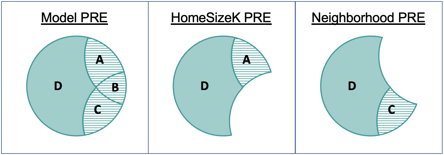
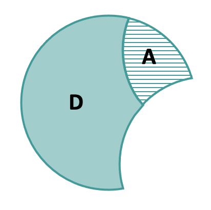
Each of these Venn diagrams represents a specific PRE as the striped area divided by the area of the entire shape.
The PRE for the multivariate model is 0.54. This tells us the proportion of error that is reduced by the overall model compared with the empty model. The PRE for HomeSizeK (0.29) tells us the error reduced by HomeSizeK over and above the neighborhood model. The PRE for Neighborhood (.021) similarly is the error reduced by adding Neighborhood over and above the home size model.
F for Targeted Model Comparisons
As with single-predictor models, the F for HomeSizeK is calculated as the ratio of two variances (aka, MS, or Mean Square Error). This time, however, it is the ratio of MS for HomeSizeK (42004, which is the variance exclusively reduced by HomeSizeK) divided by the MS Error (3613).
Analysis of Variance Table (Type III SS)
 Model: PriceK ~ Neighborhood + HomeSizeK

                                        SS df        MS      F    PRE     p
 ------------ --------------- | ---------- -- --------- ------ ------ -----
        Model (error reduced) | 124402.900  2 62201.450 17.216 0.5428 .0000
 Neighborhood                 |  27758.138  1 27758.138  7.683 0.2094 .0096
    HomeSizeK                 |  42003.739  1 42003.739  11.626 0.2862 .0019
        Error (from model)    | 104774.201 29  3612.903
 ------------ --------------- | ---------- -- --------- ------ ------ -----
        Total (empty model)   | 229177.101 31  7392.810
As you can see in the ANOVA table, the F for HomeSizeK is 11.63. As we have noted before, F is related to PRE, but expresses the strength of the predictor per degree of freedom expended to achieve that strength.
\[F_{HomeSize} = \frac{MS_{HomeSize}}{MS_{Error}}\]
Each MS is the SS divided by the degrees of freedom (df). The MS for HomeSizeK is based on the SS for HomeSizeK divided by the df for HomeSizeK. The df for HomeSizeK is 1 because only one additional parameter has been estimated in order to include HomeSizeK in the model.
Each Row in the ANOVA Table Represents a Comparison of Two Models
There is a handy R function called generate_models() that takes as its input a multivariate model and outputs all the model comparisons that can be made in relation to that model. Try it in the code block below.
require(coursekata)

# delete when coursekata-r updated
Smallville <- read.csv("https://docs.google.com/spreadsheets/d/e/2PACX-1vTUey0jLO87REoQRRGJeG43iN1lkds_lmcnke1fuvS7BTb62jLucJ4WeIt7RW4mfRpk8n5iYvNmgf5l/pub?gid=1024959265&single=true&output=csv")
Smallville$Neighborhood <- factor(Smallville$Neighborhood)
Smallville$HasFireplace <- factor(Smallville$HasFireplace)
# this saves the multivariate model
multi_model <- lm(PriceK~ Neighborhood + HomeSizeK, data = Smallville)

# write code to generate the model comparisons
multi_model <- lm(PriceK~ Neighborhood + HomeSizeK, data = Smallville)
generate_models(multi_model)
# temporary SCT
ex() %>% check_error()── Comparison Models for Type III SS ───────────────────────────────────────────
── Full Model
complex: PriceK~ Neighborhood + HomeSize
simple: PriceK~ NULL
── Neighborhood
complex: PriceK~ Neighborhood + HomeSize
simple: PriceK~ HomeSize
── HomeSize
complex: PriceK~ Neighborhood + HomeSize
simple: PriceK~ Neighborhood