Chapter 6 - Quantifying Error
6.1 Quantifying Total Error Around a Model
Up to now we have developed the idea that a statistical model can be thought of as a number—a predicted value for the outcome variable. We are trying to model the Data Generating Process (DGP). But because we can’t see the DGP directly, we fit a model to our data, estimating the parameters.
Using the DATA = MODEL + ERROR framework, we have defined error as the residual that is left after we take out the model. In the case of our simple model for a quantitative outcome variable, the model is the mean, and the error— or residual—is the deviation of each score above or below the mean.
We represent the simple model like this using the notation of the General Linear Model:
\[Y_{i}=b_{0}+e_{i}\]
This equation represents each score in our data as the sum of two components: the mean of the distribution (represented by \(b_{0}\)), and the deviation of that score above or below the mean (represented as \(e_{i}\)). In other words, DATA = MODEL + ERROR.
In this chapter, we will dig deeper into the ERROR part of our DATA = MODEL + ERROR framework. In particular, we will develop methods for quantifying the total amount of error around a model, and for modeling the distribution of error itself.
Quantifying the total amount of error will help us compare models to see which one explains more variation. Modeling the distribution of error will help us to make more detailed predictions about future observations and more precise statements about the DGP.
At the outset, it is worth remembering what the whole statistical enterprise is about: explaining variation. Once we have created a model, we can think about explaining variation in a new way, as reducing error around the model.
We have noted before that the mean is a better model of a quantitative outcome variable when the spread of the distribution is smaller than when it is larger. When the spread is smaller, the residuals from the model are smaller. Quantifying the total error around a model will help us to know how good our models are, and which models are better than others.
To make this concrete, let’s consider our very simple model of our tiny sample (n = 6) of data, TinyFingers. Here is the data frame including the Predictions and Residuals from the Tiny_empty_model.
StudentID Thumb Prediction Residual
1 1 56 62 -6
2 2 60 62 -2
3 3 61 62 -1
4 4 63 62 1
5 5 64 62 2
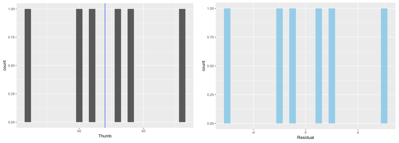
6 6 68 62 6The histograms below show the distribution of Thumb and the distribution of Residual for our tiny data set. And of course, as you know by now, these distributions have the exact same shape, but different means.
It makes sense to use residuals to analyze error from the model. If we want to quantify total error, why not just add up all the residuals? Worse models should have more error, so the sum of all the errors should represent the “total” error, right?
Let’s do that, using one of the first R functions you learned, sum(). The following code will add up all the residuals from our Tiny_empty_model.
sum(TinyFingers$Residuals)[1] 0Although we might at first think that the sum of the residuals would be a good indicator of total error, we discovered a fatal flaw in that approach in the previous chapter: the sum of the residuals around the mean is equal to 0! If this were our measure of total error, all data sets would be equally well modeled by the mean, because the residuals around the mean would always sum to 0. Thus a data set widely spread out around the mean, and one tightly clustered around the mean, would have the same amount of error around this simple model. Clearly we need a different approach.
Statisticians have explored various methods for quantifying error around a mean. Two of the most common, which we will discuss here are Sum of Absolute Deviations (SAD), and Sum of Squared Deviations (SS). Each provides a different way of solving the problem created by simply summing residuals. Let’s take a look at each.
Sum of Absolute Deviations (SAD)
Sum of absolute deviations gets around the problem that deviations around the mean always add up to 0 by taking the absolute value of the deviations. We can represent this summary measure like this:
\[\sum_{i=1}^n |Y_i-\bar{Y}|\]
In this context, “deviations from the mean” means the same thing as “residuals from the empty model,” given that the mean is our model. We already have the deviations of each thumb length from the mean in the Residual column of TinyFingers.
We can take the absolute value of each deviation from the mean by using the function abs().
abs(TinyFingers$Residual)[1] 6 2 1 1 2 6As with everything, if we don’t save it, these absolute values of the residuals are lost. Modify the following code to save the absolute residuals in the variable AbsResidual in TinyFingers. Then use sum() to sum up the AbsResidual.
require(coursekata)

TinyFingers <- data.frame(
    StudentID = 1:6,
    Thumb = c(56, 60, 61, 63, 64, 68)
)
Tiny_empty_model <- lm(Thumb ~ NULL, data = TinyFingers)
TinyFingers <- TinyFingers %>% mutate(
    Predicted = predict(Tiny_empty_model),
    Residual = resid(Tiny_empty_model)
)
# save the absolute residuals to AbsResidual
TinyFingers$AbsResidual <-

# modify this code to sum up AbsResidual
sum()
TinyFingers$AbsResidual <- abs(TinyFingers$Residual)
sum(TinyFingers$AbsResidual)
ex() %>% {
    check_object(., "TinyFingers") %>% check_column("AbsResidual") %>% check_equal()
    check_function(., "sum") %>% check_result() %>% check_equal()
}[1] 18Sum of Squared Deviations (SS)
Another way to quantify error, which gets around the problem of the sum of deviations adding up to 0, is to square the deviations (i.e., residuals). This approach is represented like this:
\[\sum_{i=1}^n (Y_i-\bar{Y})^2\]
Since we already have the column Residual, we can easily create a column of squared residuals. We don’t need to use absolute value here because squaring will result in a positive value no matter the starting value. In R, we represent exponents with the caret symbol (^, usually above the 6 on a standard keyboard).
TinyFingers$Residual^2[1] 36 4 1 1 4 36Try it for yourself. Save the squared residuals in the variable SqrResidual in TinyFingers. Then use sum() to sum up the SqrResidual.
require(coursekata)

TinyFingers <- data.frame(
    StudentID = 1:6,
    Thumb = c(56, 60, 61, 63, 64, 68)
)
Tiny_empty_model <- lm(Thumb ~ NULL, data = TinyFingers)
TinyFingers <- TinyFingers %>% mutate(
    Predicted = predict(Tiny_empty_model),
    Residual = resid(Tiny_empty_model)
)
# save the squared residuals to SqrResidual
TinyFingers$SqrResidual <-

# modify this code to sum up SqrResidual
sum()
TinyFingers$SqrResidual <- TinyFingers$Residual^2
sum(TinyFingers$SqrResidual)
ex() %>% {
    check_object(., "TinyFingers") %>% check_column("SqrResidual") %>% check_equal()
    check_function(., "sum") %>% check_result() %>% check_equal()
}[1] 82Each of these measures has been used by statisticians. But when the mean is the model, sum of squares has prevailed. Here is a little video with Dr. Ji regarding why.
If you want to try it yourself, here is a link to the sum of squares applet, and below are the data you can copy/paste into the little “sample data” box. (Here’s the full link in case that one doesn’t work: http://www.rossmanchance.com/applets/RegShuffle.htm)
| StudentID | Thumb |
| 1 | 56 |
| 2 | 60 |
| 3 | 61 |
| 4 | 63 |
| 5 | 64 |
| 6 | 68 |