6.6 Modeling the Shape of the Error Distribution
We quantify error because, fundamentally, it tells us how well our model fits the data. When our model is the mean, calculations of SS, variance, and standard deviation are useful because these are all minimized at the mean. And minimizing error is our number one priority as statisticians. The less error, the more variation is explained by the model.
Quantifying error also gives us a way to put deviations in perspective. No matter what the scale of measurement is on an outcome variable, standard deviation is a convenient way of assessing how far particular scores are above or below the mean—especially when it is incorporated into a z score.
But as useful as it is to quantify how much error there is, it is also useful to model the shape of the distribution of error—especially if we want to make better predictions about future randomly sampled observations.
Although the mean is the best point estimate of the mean of the DGP, and the best predictor of a future observation if we must choose a single number, we can make more accurate predictions if we are willing to make some assumptions about the shape of the distribution of error in the population.
For example, if we are willing to assume that the distribution of a variable in the population is symmetrical around the mean, then we can predict that there is a .5 probability that the next observation will be above the mean, and a .5 chance that it will be below the mean.
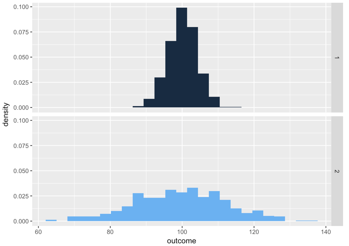
Take a look at the two sample distributions above. The mean of both distributions is 100. Because they both appear roughly symmetrical, let’s assume that the DGP that produced each distribution would, in the long term, produce a perfectly symmetrical population distribution.
If we assume that both of the DGPs produce symmetrical distributions, then both are equally likely to produce a next observation that is greater than the mean. Some people might say the DGP for Sample 2 is more likely to produce an observation above the mean, because that DGP is more likely to produce a larger number than the DGP for Sample 1. But note: it’s also more likely to produce a smaller number than the DGP for Sample 1. Both distributions have a 50% chance of producing a next observation above the mean.
If we are willing to make more detailed assumptions about the shapes of the distributions, we can use those assumptions to calculate the probability not just of the next observation being above or below the mean, but also the probability of the next observation being greater than, or less than, any other score—not just the mean.
This time the answer is different. You would be more confident in getting a score higher than 110 if your data distribution were the one on the bottom, precisely because there is more error (and a wider spread) in Sample 2. A fairly large proportion of scores in Sample 2 are above 110, whereas a much smaller proportion are above 110 in Sample 1.
But what if you wanted to calculate the probability that the next observation would be greater than 110?
To answer this question, we need to model the shape of the distribution of error. Specifically, we need a probability distribution—something that will allow us to estimate the probability of a particular event, just as the rectangles and triangles gave us a way to estimate the area of the State of California.
Calculating Probabilities From the Distribution of Data
One way to get this probability distribution is to use the distribution of data. Recall that we used the mean of a distribution of data as an estimate for the mean of the population. In similar fashion, we can use the proportion of cases that fall within a certain region in our data to estimate the probability that the DGP would produce a next observation in that region.
Let’s use R to count the proportion of observations in each of the samples above with values greater than 110 on the outcome variable. First, we create a TRUE or FALSE variable (a Boolean variable) to record whether each value on the outcome variable is greater than 110.
Here is the code to do that for a data frame called sample_2, which holds the data for Sample 2 shown in the histogram above.
sample_2$greater_than_110 <- sample_2$outcome > 110We will use a combination of functions to look at a few lines of the data frame sample_2, zeroing in on just the columns outcome and greater_than_110.
head(select(sample_2, outcome, greater_than_110)) outcome greater_than_110
1 100.92764 FALSE
2 96.43758 FALSE
3 85.80109 FALSE
4 100.13551 FALSE
5 111.89921 TRUE
6 119.12761 TRUEIt’s always a good idea to look at the data to make sure your code did what you thought it was going to do. In this case, it looks like it did. You can see that for row one, the value of outcome was 100.92764, which is less than 110, and the value for greater_than_110 is FALSE. That lines up. Row 6 has a value of outcome that is greater than 110, and sure enough, it has TRUE as its value for greater_than_110.
Next, we need to get a tally of these TRUEs and FALSEs. Write code to get the tally of greater_than_110 (both as a frequency and as a proportion).
require(coursekata)

# do not remove setup code here even though sample_1 isn't used!
# it is important to call set.seed(1) and rnorm both times so that the tally matches the figures in the text
set.seed(1)
sample_1 <- data.frame(
    outcome = rnorm(500, 100, 4),
    explanatory = rep(1, 100)
)
sample_2 <- data.frame(
    outcome = rnorm(500, 100, 12),
    explanatory = rep(2, 100)
)
sample_2$greater_than_110 <- sample_2$outcome > 110
# get a tally of greater_than_110 in sample_2
tally()

# get the tally in proportions
tally()
tally(~greater_than_110, data = sample_2)
tally(~greater_than_110, data = sample_2, format = "proportion")
ex() %>% {
    check_function(., "tally", index = 1) %>% check_result() %>% check_equal()
    check_function(., "tally", index = 2) %>% check_result() %>% check_equal()
}greater_than_110
TRUE FALSE
101 399greater_than_110
TRUE FALSE
0.202 0.798Trying It Out With Fingers
Let’s apply these ideas to the empty_model that we created before from the Fingers data frame. In that empty model, we modeled thumb lengths as the mean (60.1 mm) plus error. The error can either be modeled as the residuals around the mean, or as the variation around the mean. In either case, the distribution is the same, except that when we model the residuals the mean is going to be 0.
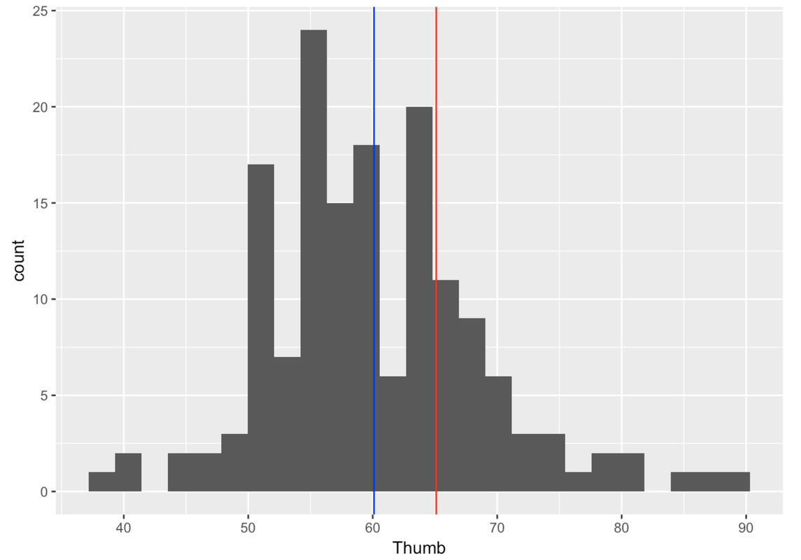
Use the distribution of Thumb in the Fingers data frame as a probability model of the DGP. Then, write the R code to calculate the likelihood of a student having a thumb length longer than 65.1 mm.
require(coursekata)
# modify this to create a boolean variable that records whether a Thumb is greater than 65.1
Fingers$GreaterThan65.1 <-

# modify this to find the proportion of GreaterThan65.1
tally(~ , data = , format = "proportion")
Fingers$GreaterThan65.1 <- Fingers$Thumb > 65.1
tally(~GreaterThan65.1, data = Fingers, format = "proportion")
ex() %>% {
    check_object(., "Fingers") %>% check_column("GreaterThan65.1") %>% check_equal()
    check_function(., "tally") %>% check_result() %>% check_equal()
}GreaterThan65.1
TRUE FALSE
0.1974522 0.8025478We can see from the output that approximately .20 of students’ thumbs are longer than 65.1 mm. Based on this, we would estimate that if another student were randomly selected and added to this data set, the likelihood that his/her thumb would be longer than 65.1 would be .20.