8.7 Assessing Model Fit with PRE and F
Comparing PRE for the Two Models
Let’s go back to our supernova output for the Height2Group and Height models.
Height2Group Model
Analysis of Variance Table (Type III SS)
Model: Thumb ~ Height2Group

                               SS  df      MS      F    PRE     p
----- --------------- | --------- --- ------- ------ ------ -----
Model (error reduced) |   830.880   1 830.880 11.656 0.0699 .0008
Error (from model)    | 11049.331 155  71.286
----- --------------- | --------- --- ------- ------ ------ -----
Total (empty model)   | 11880.211 156  76.155
Height Model
Analysis of Variance Table (Type III SS)
Model: Thumb ~ Height

                               SS  df       MS      F    PRE     p
----- --------------- | --------- --- -------- ------ ------ -----
Model (error reduced) |  1816.862   1 1816.862 27.984 0.1529 .0000
Error (from model)    | 10063.349 155   64.925
----- --------------- | --------- --- -------- ------ ------ -----
Total (empty model)   | 11880.211 156   76.155
PRE has the same interpretation in the context of regression models as it does for the group models. As we have pointed out, the total sum of squares is the same for both models. And the PRE is obtained in both cases by dividing SS Model by SS Total.
The main difference between the two models is in the way that error is conceptualized. In the two-group model, error is the deviations of each score from its group mean; in the regression model, error is the deviation of each score from its predicted score on the regression line. But underneath it all, error in both cases is simply the residual between the score predicted by the model and the actual observed score for each student.
Many statistics textbooks emphasize the difference between ANOVA models (such as our two- and three-group models) and regression models (such as our Height model). But in fact, the two types of models are fundamentally the same and easily incorporated into the General Linear Model framework.
Because the differences between these models have been stressed, the PRE statistic has been given different names in the two traditions. As we noted earlier, PRE in the context of ANOVA has been called \(\eta^2\) (eta-squared). In the context of regression, PRE is usually referred to as \(R^2\) (R-squared). For the simple models we are considering, no matter what you call it, the interpretation of PRE is identical: proportion reduced error of the model compared with the empty model. Or, put another way, proportion variation explained.
Using the F Ratio for Comparing Models
Finally, we can also assess model fit by looking at the F ratio, which we first discussed in Chapter 7. Whereas PRE is a proportion based on sums of squares, the F ratio is based on mean squares or MS (commonly called variance). Variance takes the SS and divides by df. Thus, it indicates how much we have reduced error compared with the empty model per degree of freedom spent.
More on F Versus PRE
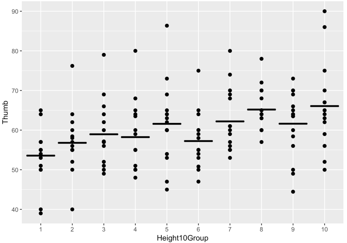
To get a more concrete idea of why this matters, let’s compare yet another group model to the Height model, the Height10Group model. We will run the following R code to create a new grouping variable called Fingers$Height10Group, and then make it a factor. Height10Group divides the Fingers sample into 10 equally-sized groups based on Thumb.
Fingers$Height10Group <- ntile(Fingers$Height, 10)
Fingers$Height10Group <- factor(Fingers$Height10Group)
Below is a jitter plot of the 10 groups, with a horizontal line representing the mean of each group.
We next used the following code to fit a group model of Thumb using Height10Group, and produce an ANOVA table for the Height10Group model.
Height10Group_model <- lm(Thumb ~ Height10Group, data = Fingers)
supernova(Height10Group_model)
Below are the supernova() tables for three models: Height2Group, Height10Group, and Height. The outcome variable for all three models, again, is Thumb.
Height2Group Model
Analysis of Variance Table (Type III SS)
Model: Thumb ~ Height2Group

                               SS  df      MS      F    PRE     p
----- --------------- | --------- --- ------- ------ ------ -----
Model (error reduced) |   830.880   1 830.880 11.656 0.0699 .0008
Error (from model)    | 11049.331 155  71.286
----- --------------- | --------- --- ------- ------ ------ -----
Total (empty model)   | 11880.211 156  76.155
Height10Group Model
Analysis of Variance Table (Type III SS)
Model: Thumb ~ Height10Group

                               SS  df      MS     F    PRE     p
----- --------------- | --------- --- ------- ----- ------ -----
Model (error reduced) |  1920.474   9 213.386 3.149 0.1617 .0017
Error (from model)    |  9959.737 147  67.753
----- --------------- | --------- --- ------- ----- ------ -----
Total (empty model)   | 11880.211 156  76.155
Height Model
Analysis of Variance Table (Type III SS)
Model: Thumb ~ Height

                               SS  df       MS      F    PRE     p
----- --------------- | --------- --- -------- ------ ------ -----
Model (error reduced) |  1816.862   1 1816.862 27.984 0.1529 .0000
Error (from model)    | 10063.349 155   64.925
----- --------------- | --------- --- -------- ------ ------ -----
Total (empty model)   | 11880.211 156   76.155
To look at how many degrees of freedom are used by a model, look at the df column in the row that says “Model (error reduced).” Notice that the Height10Group model spends more degrees of freedom (nine) compared to the other two models (they each just spend one).
Now, what do we get for our degrees of freedom? When we go from the Height2Group model to the Height model, PRE goes up from .07 to .15 without spending any additional degrees of freedom. That seems like a no brainer!
The Height10Group model produces the highest PRE of all the models (.18), but look what we give up: eight additional degrees of freedom. A model that consists of 10 group mean predictions is not very elegant compared to one with just a y intercept and slope. Here’s what the Height10Group model would look like in GLM notation:
\(Y_i=b_0+b_{1}X_{1i}+b_{2}X_{2i}+b_{3}X_{3i}+b_{4}X_{4i}+\)\(b_{5}X_{5i}+b_{6}X_{6i}+b_{7}X_{7i}+b_{8}X_{8i}+b_{9}X_{9i}+e_i\)
Compare that jumble of symbols with the Height model:
\[b_0+b_{1}X_{i}\]
That’s a truly elegant model! True, it doesn’t reduce error as much as the Height10Group model. But because the regression model only uses one degree of freedom beyond the empty model, it’s a bargain, adding a lot of explanatory power without sacrificing simplicity or elegance.
Comparing F Ratios for the Three Models
The supernova() function also calculated the F ratio for each of the three models. As we can see from the table below, the F ratio paints a different picture of the three models than we get by looking only at PRE.
| Model (Group) | PRE | F Ratio |
|---|---|---|
| Height2Group Model | .0699 | 11.656 |
| Height10Group Model | .1617 | 3.149 |
| Height Model | .1529 | 27.984 |
Going by PRE alone, the Height10Group model would appear to be the best one. But when we use F, which incorporates degrees of freedom into our calculation, the Height model is the clear winner, with an F of 27.984. The Height10Group model is by far the worst, with an F of 3.149.