8.8 Correlation
You might have heard of Pearson’s r, often referred to as a “correlation coefficient.” Correlation is just a special case of regression in which both the outcome and explanatory variables are transformed into z scores prior to analysis.
Let’s see what happens when we transform the two variables we have been working with: Thumb length and Height. Because both variables are transformed into z scores, the mean of each distribution will be 0, and the standard deviation will be 1. The function zscore() will convert all the values in a variable to z scores.
require(coursekata)

Fingers <- filter(Fingers, Thumb >= 33 & Thumb <= 100)
Height.model <- lm(Thumb ~ Height, data = Fingers)
Fingers$Height.resid <- resid(Height.model)
# this transforms all Thumb lengths into zscores
Fingers$zThumb <- zscore(Fingers$Thumb)

# modify this to do the same for Height
Fingers$zHeight <-
# this transforms all Thumb lengths into zscores
Fingers$zThumb <- zscore(Fingers$Thumb)

# modify this to do the same for Height
Fingers$zHeight <- zscore(Fingers$Height)
ex() %>% check_object("Fingers") %>% {
    check_column(., "zThumb") %>% check_equal()
    check_column(., "zHeight") %>% check_equal()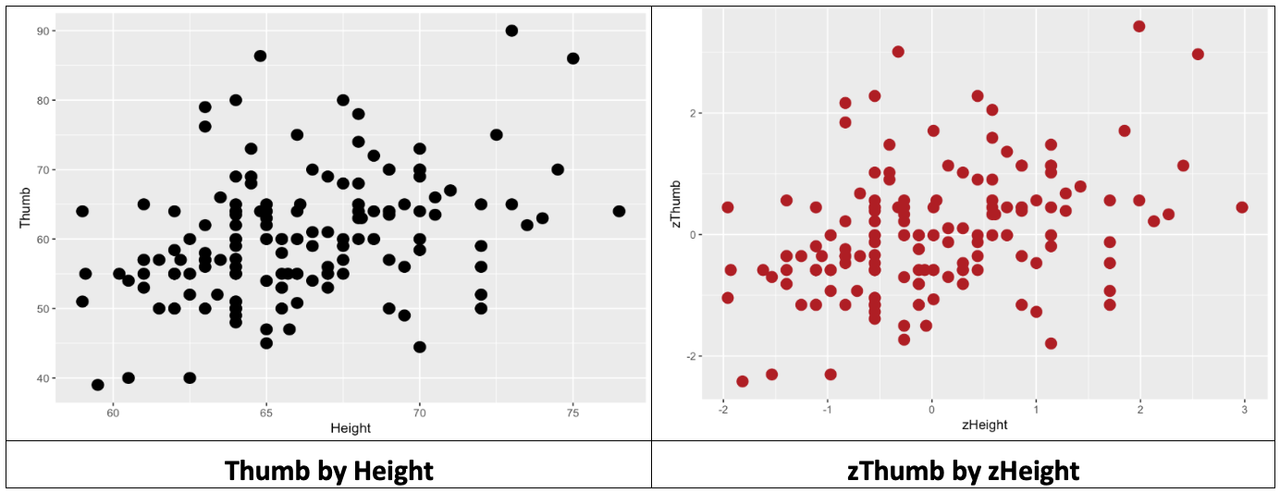
}Let’s make a scatterplot of zThumb and zHeight and look at the distribution. Then also make (again) a scatterplot of Thumb and Height, and compare the two scatterplots.
Make two scatterplots by modifying the code below.
require(coursekata)

Fingers <- Fingers %>%
    filter(Thumb >= 33 & Thumb <= 100) %>%
    mutate(
        zThumb = zscore(Thumb),
        zHeight = zscore(Height)
    )
Height.model <- lm(Thumb ~ Height, data = Fingers)
# this makes a scatterplot of the raw scores
# size makes the points bigger or smaller
gf_point(Thumb ~ Height, data = Fingers, size = 4, color = "black")

# modify this to make a scatterplot of the zscores
# feel free to change the colors
gf_point( , data = Fingers, size = 4, color = "firebrick")
# this makes a scatterplot of the raw scores
 # size makes the points bigger or smaller
 gf_point(Thumb ~ Height, data = Fingers, size = 4, color = "black")

 # modify this to make a scatterplot of the zscores
 # feel free to change the colors
 gf_point(zThumb ~ zHeight, data = Fingers, size = 4, color = "firebrick")
ex() %>% {
    check_function(., "gf_point", index = 1) %>% {
        check_arg(., "object") %>% check_equal()
        check_arg(., "data") %>% check_equal()
    }
    check_function(., "gf_point", index = 2) %>% {
        check_arg(., "object") %>% check_equal()
        check_arg(., "data") %>% check_equal()
    }
}
Fitting the Regression Model to the Two Distributions
In the code window below we’ve provided the code to fit a regression line for Thumb based on Height. Below that code, fit a regression model to the two transformed variables, using zThumb as the outcome variable (instead of Thumb) and zHeight as the explanatory variable (instead of Height). Save the model in an R object called zHeight_model.
Then, print the model estimates for both the zHeight_model and the Height_model.
require(coursekata)

Fingers <- Fingers %>%
    filter(Thumb >= 33 & Thumb <= 100) %>%
    mutate(
        zThumb = zscore(Thumb),
        zHeight = zscore(Height)
    )
Height_model <- lm(Thumb ~ Height, data = Fingers)
# this fits a regression model of Thumb by Height
Height_model <- lm(Thumb ~ Height, data = Fingers)

# modify this to fit a regression model predicting zThumb with zHeight
zHeight_model <- lm()

# this prints the estimates
Height_model
zHeight_model
zHeight_model <- lm(zThumb ~ zHeight, data = Fingers)
ex() %>% check_object("zHeight_model") %>% check_equal()Next, redo the two scatterplots, this time overlaying the best-fitting regression line for each one.
require(coursekata)

Fingers <- Fingers %>%
    filter(Thumb >= 33 & Thumb <= 100) %>%
    mutate(
        zThumb = zscore(Thumb),
        zHeight = zscore(Height)
    )
Height.model <- lm(Thumb ~ Height, data = Fingers)
# this overlays the best-fitting regression model on this scatterplot
gf_point(Thumb ~ Height, data = Fingers, size = 4, color = "black") %>%
    gf_lm()

# modify this to overlay the best-fitting regression model on this scatterplot
gf_point(zThumb ~ zHeight, data = Fingers, size = 4, color = "firebrick")
# this overlays the best-fitting regression model on this scatterplot
gf_point(Thumb ~ Height, data = Fingers, size = 4, color = "black") %>%
    gf_lm()

# modify this to overlay the best-fitting regression model on this scatterplot
gf_point(zThumb ~ zHeight, data = Fingers, size = 4, color = "firebrick") %>%
    gf_lm()
ex() %>% check_function("gf_lm", index = 2)Below we’ve organized the results of all this in a table: the two scatterplots, best-fitting regression lines, and estimated model parameters.
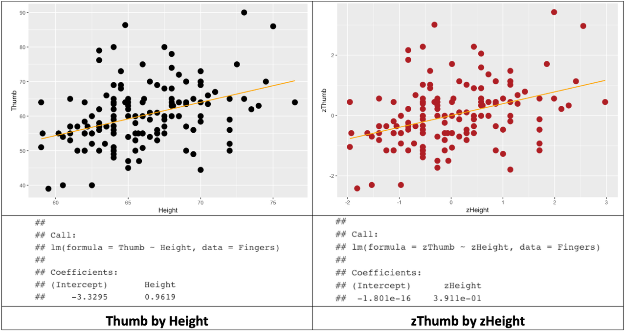
Note that R will sometimes express parameter estimates in scientific notation. Thus, -1.801e-16 means that the decimal point is shifted 16 digits to the left. So, the actual y-intercept of the best-fitting regression line is -.00000000000000018. Which is, for all practical purposes, 0.
We know from earlier that the best-fitting regression line passes through the mean of both the outcome and explanatory variables. Note that in the case of zThumb and zHeight, the middle of the scatterplot is at 0 on both the x- and y-axes. The y-intercept is 0 in this model because when x is 0, y is also 0.
Comparing the Fit of the Two Models
Let’s now run supernova() on the two models, and compare their fit to the data.
require(coursekata)

Fingers <- Fingers %>%
    filter(Thumb >= 33 & Thumb <= 100) %>%
    mutate(
        zThumb = zscore(Thumb),
        zHeight = zscore(Height)
    )
Height_model <- lm(Thumb ~ Height, data = Fingers)
zHeight_model <- lm(zThumb ~ zHeight, data = Fingers)
# this quantifies error from Height_model
supernova(Height_model)

# modify this to quantify error from zHeight_model
supernova()
# this quantifies error from Height_model
supernova(Height_model)

# modify this to quantify error from zHeight_model
supernova(zHeight_model)
ex() %>% check_output_expr("supernova(zHeight_model)")Analysis of Variance Table (Type III SS)
Model: Thumb ~ Height
SS df MS F PRE p
----- --------------- | --------- --- -------- ------ ------ -----
Model (error reduced) | 1816.862 1 1816.862 27.984 0.1529 .0000
Error (from model) | 10063.349 155 64.925
----- --------------- | --------- --- -------- ------ ------ -----
Total (empty model) | 11880.211 156 76.155 Analysis of Variance Table (Type III SS)
Model: zThumb ~ zHeight
SS df MS F PRE p
----- --------------- | ------- --- ------ ------ ------ -----
Model (error reduced) | 23.857 1 23.857 27.984 0.1529 .0000
Error (from model) | 132.143 155 0.853
----- --------------- | ------- --- ------ ------ ------ -----
Total (empty model) | 156.000 156 1.000 The fit of the models is identical because all we have changed is the unit in which we measure the outcome and explanatory variables. We saw when we first introduced z scores that transforming an entire distribution into z scores did not change the shape of the distribution, but only the mean and standard deviation (to 0 and 1).
The same thing is true when we transform both the outcome and explanatory variables. The z transformation does not change the shape of the bivariate distribution, as represented in the scatterplot, at all. It simply changes the scale on both axes to standard deviations instead of inches and millimeters.
Unlike PRE, which is a proportion of the total, SS are expressed in the units of the measurement. So if we converted the mm (for Thumb length) and inches (for Height) into cm, feet, etc, the SS would change to reflect those new units.