4.9 From Categorical to Quantitative Explanatory Variables
Okay, let’s go back to where we were, explaining the variation in thumb length using the variable Sex.
THUMB LENGTH = SEX + OTHER STUFF
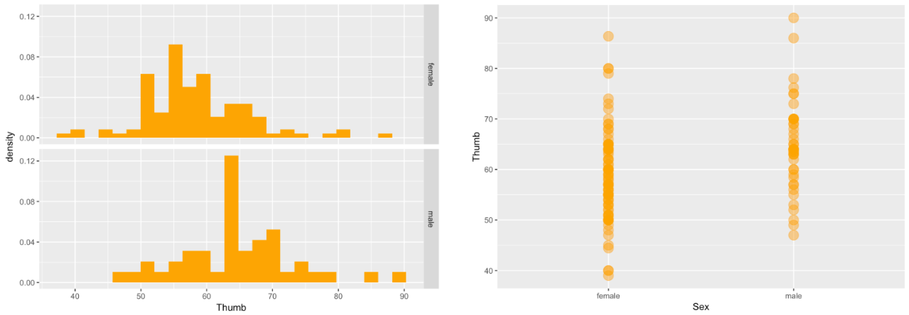
Let’s look at the histograms and scatterplots of this word equation, which showed that the overall variation in Thumb length could be partially explained by taking Sex into account.
gf_dhistogram( ~ Thumb, data = Fingers, fill = "orange") %>%
  gf_facet_grid(Sex ~ .)
gf_point(Thumb ~ Sex, data = Fingers, color = "orange", size = 5, alpha = .5)
Let’s now see if we can take the same approach for a different explanatory variable: Height. First, let’s write a word equation to represent the relationship we want to explore:
THUMB LENGTH = HEIGHT + OTHER STUFF
We might expect that people who are taller have longer thumbs.
We actually could use the same approach with Height as we did with Sex. But notice, whereas Sex is a categorical variable, Height is continuous. We can construct a new categorical variable by cutting up Height into two categories—short and tall. You can do that using the function ntile().
Recall that quartiles could be created by sorting a quantitative variable in order and then dividing the observations into four groups of equal sizes. In the same way, we could create tertiles (three equal-sized groups), quantiles (five groups), deciles (10 groups), and so on. The ntile() function lets you divide observations into any (n) number of groups (-tiles).
Running the code below will divide the students into two equal groups: those taller than the middle student, and those shorter. Students who belong to the shorter group will get a 1 and those in the taller group will get a 2.
ntile(Fingers$Height, 2) [1] 2 1 1 2 2 2 2 2 1 1 2 2 1 2 1 1 2 2 1 2 1 1 1 2 1 1 2 2 1 2 1 2 1 1 1 1 1
[38] 2 1 2 1 1 2 2 1 1 1 2 1 1 1 2 1 1 2 1 2 1 1 2 1 1 1 2 1 2 2 2 2 2 2 2 2 2
[75] 1 2 1 1 2 1 1 1 1 2 2 2 1 2 1 1 1 2 1 2 1 2 1 2 2 2 2 1 1 1 2 2 1 1 2 1 1
[112] 2 2 2 2 1 2 2 2 2 2 2 1 1 1 2 1 2 2 1 1 1 2 2 2 1 1 2 1 1 1 2 2 2 1 1 1 2
[149] 1 2 2 2 2 1 1 1 2Like everything else in R, if you don’t save it to a data frame, this work will go to waste. Use ntile() to create the shorter and taller group but this time, save this in Fingers as a new variable called Height2Group.
require(coursekata)
# Use ntile() to cut Height into groups
Fingers$Height2Group <-

# This prints out the first 6 observations of Height and Height2Group
head(select(Fingers, Height, Height2Group))
# Use ntile() to cut Height into groups
Fingers$Height2Group <- ntile(Fingers$Height, 2)

# This prints out the first 6 observations of Height and Height2Group
head(select(Fingers, Height, Height2Group))
ex() %>% check_correct(
    check_object(., "Fingers") %>%
        check_column("Height2Group") %>%
        check_equal(),
    {
        check_error(.)
        check_function(., "ntile", not_called_msg = "Have you called ntile()?") %>%
            check_arg("n") %>%
            check_equal()
    }
)

incorrect_msg <- "Did you remember to use select() to select the Height and Height2Group columns from the Fingers data frame before calling head()?"
ex() %>%  check_or(
    check_output_expr(., "head(select(Fingers, Height, Height2Group))", missing_msg = incorrect_msg),
    check_output_expr(., "head(select(Fingers, Height2Group, Height))", missing_msg = incorrect_msg)
) Height Height2Group
1 70.5 2
2 64.8 1
3 64.0 1
4 70.0 2
5 68.0 2
6 68.0 2Now we can try looking at the data the same way as we did for Sex, which also had two levels.
Create histograms in a grid to look at variability in Thumb based on Height2Group.
require(coursekata)
# Here we create the variable Height2Group
Fingers$Height2Group <- ntile(Fingers$Height, 2)

# Try creating histograms of Thumb in a grid by Height2Group
# Here we create the variable Height2Group
Fingers$Height2Group <- ntile(Fingers$Height, 2)

# Try creating histograms of Thumb in a grid by Height2Group
gf_histogram(~Thumb, data=Fingers) %>%
    gf_facet_grid(Height2Group ~ .)
ex() %>% check_or(
    check_function(., "gf_histogram") %>% {
        check_arg(., "object") %>% check_equal()
        check_arg(., "data") %>% check_equal()
    },
    override_solution(., "gf_histogram(Fingers, ~Thumb)") %>%
        check_function("gf_histogram") %>% {
            check_arg(., "object") %>% check_equal()
            check_arg(., "gformula") %>% check_equal()
        }
)


ex() %>%
    check_function(., "gf_facet_grid", not_called_msg = "Have you called gf_facet_grid() to put your histograms in a grid?") %>%
    check_arg(., "object") %>%
    check_equal()


ex() %>% check_or(
    check_function(., "gf_facet_grid") %>%
        check_arg(2) %>%
        check_equal(),
    override_solution(., "gf_facet_grid(gf_histogram(Fingers, ~Thumb), . ~ Height2Group)") %>%
        check_function('gf_facet_grid') %>%
        check_arg(2) %>%
        check_equal()
)
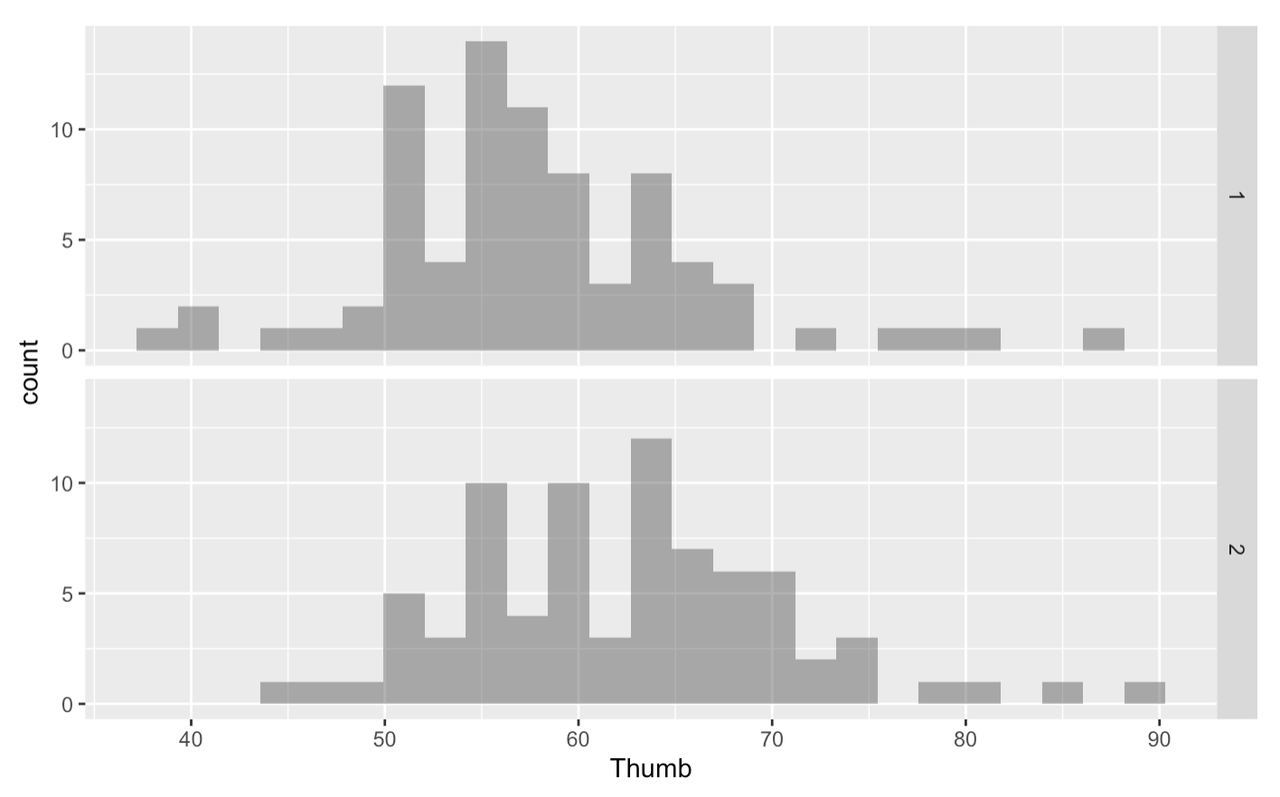
Is there a difference between groups 1 and 2? Does the taller group have longer thumbs than the shorter group? It would be more helpful if instead of groups 1 and 2, these visualizations were labeled “short” and “tall”.
The variable Height2Group is categorical because the numbers are stand-ins for categories. In this case, the number 1 stands for “short”. This differs from quantitative variables for which the numbers actually stand for quantities. For instance, in the variable Thumb, 60 stands for 60 mm.
Before, we learned to use the factor() function to turn a numeric variable into a factor: factor(Fingers$Height2Group). We can use the same function to label the levels of a categorical variable.
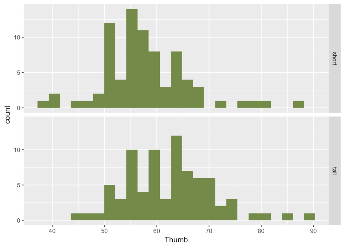
factor(Fingers$Height2Group, levels = c(1,2), labels = c("short", "tall"))This looks complicated. But you can think of the input to the factor() function as having three parts (what we call arguments): the variable name, the levels, and the labels.
As always, if we want this change to stick around, we have to save this back into a variable. Use the <- (assignment operator that looks like an arrow) to save the result of the factor() function back into Fingers$Height2Group.
require(coursekata)
# This code will cut Height from Fingers into 2 categories
Fingers$Height2Group <- ntile(Fingers$Height, 2)

# Try using factor() to label the groups "short" and "tall"


# This code recreates the faceted histogram
gf_histogram(~ Thumb, data = Fingers) %>%
gf_facet_grid(Height2Group ~ .)
Fingers$Height2Group <- ntile(Fingers$Height, 2)
Fingers$Height2Group <- factor(Fingers$Height2Group, levels = c(1,2), labels = c("short", "tall"))
gf_histogram(~ Thumb, data = Fingers) %>%
gf_facet_grid(Height2Group ~ .)
ex() %>% check_correct(
    check_object(., "Fingers") %>% check_column("Height2Group") %>% check_equal(incorrect_msg = "Did you remember to save the factored variable back into Fingers$Height2Group?"),
{
    check_error(.)
    check_function(., "factor") %>% check_arg("levels") %>% check_equal()
    check_function(., "factor") %>% check_arg("labels") %>% check_equal()

}
)


success_msg("Wow! You're a rock staR. Keep up the good work!")
To get a different perspective on the same data, let’s also try looking at these distributions with a scatterplot and boxplot.
require(coursekata)
Fingers <- supernova::Fingers %>%
    mutate(Height2Group = factor(ntile(Height, 2), 1:2, c("short", "tall")))
# Create a scatterplot of Thumb by Height2Group


# Create boxplots of Thumb by Height2Group
gf_point(Thumb ~ Height2Group, data = Fingers)

gf_boxplot(Thumb ~ Height2Group, data = Fingers)
sol_2 <- "gf_boxplot(Fingers$Thumb ~ Fingers$Height2Group)"
ex() %>% check_or(
    check_function(., "gf_boxplot") %>%
        check_result() %>% check_equal(),
    override_solution(., sol_2) %>%
    check_function(., "gf_boxplot") %>%
        check_result() %>% check_equal()
)
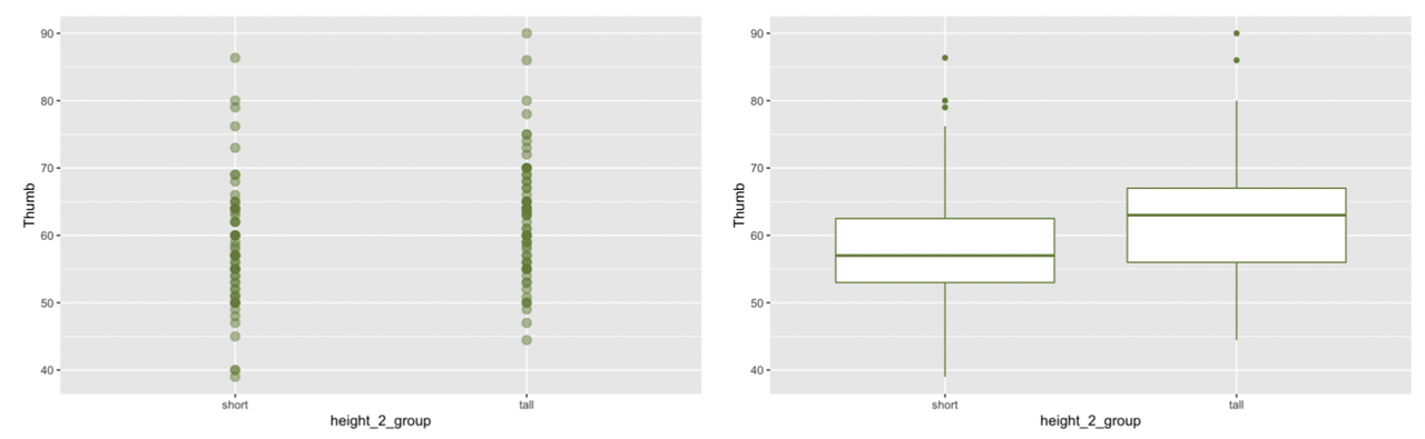
Similar to what we found for Sex, where there was a lot of variability within the female group and male group, there is a lot of variability within the short and tall groups. But there is less variability within each group than there would be in the overall distribution we would get if we just combined both groups together. Again, it is useful to think about this within-group variation as the leftover variation after explaining some of the variation with Height2Group.
See if you can break Height into three categories (let’s call it Height3Group) and then compare the distribution of height across all three categories with a scatterplot. Create boxplots as well.
require(coursekata)
Fingers <- supernova::Fingers %>%
    mutate(Height2Group = factor(ntile(Height, 2), 1:2, c("short", "tall")))
# Modify this code to break Height into 3 categories: "short", "medium", and "tall"
Fingers$Height3Group <- ntile(Fingers$Height, 2)
Fingers$Height3Group <- factor( , levels = 1:2, labels = c("short", "tall"))

# Create a scatterplot of Thumb by Height3Group

# Create boxplots of Thumb by Height3Group
Fingers$Height3Group <- ntile(Fingers$Height, 3)
Fingers$Height3Group <- factor(Fingers$Height3Group, 1:3, c("short", "medium", "tall"))

gf_point(Thumb ~ Height3Group, data = Fingers)
gf_boxplot(Thumb ~ Height3Group, data = Fingers)
ex() %>% {
    check_object(., "Fingers") %>% check_column("Height3Group") %>% check_equal(incorrect_msg = "Did you remember to use `ntile()`?")
}


ex() %>% check_or(
    check_function(., "gf_point") %>% {
    check_arg(., "object") %>% check_equal()
    check_arg(., "data") %>% check_equal()
},
    override_solution(., "gf_point(Fingers, Thumb ~ Height3Group)") %>%
    check_function("gf_point") %>% {
    check_arg(., "object") %>% check_equal()
    check_arg(., "gformula") %>% check_equal()
},
    override_solution(., "gf_point(Fingers$Thumb ~ Fingers$Height3Group)") %>%
    check_function("gf_point") %>% {
    check_arg(., "object") %>% check_equal()
},
    override_solution(., "gf_jitter(Thumb ~ Height3Group, data = Fingers)") %>%
    check_function("gf_jitter") %>% {
    check_arg(., "object") %>% check_equal()
    check_arg(., "data") %>% check_equal()
},
    override_solution(., "gf_jitter(Fingers, Thumb ~ Height3Group)") %>%
    check_function("gf_jitter") %>% {
    check_arg(., "object") %>% check_equal()
    check_arg(., "gformula") %>% check_equal()
},
    override_solution(., "gf_jitter(Fingers$Thumb ~ Fingers$Height3Group)") %>%
    check_function("gf_jitter") %>%
    check_arg("object") %>% check_equal()
    )


ex() %>% check_or(
    check_function(., "gf_boxplot") %>% {
    check_arg(., "object") %>% check_equal()
    check_arg(., "data") %>% check_equal()
},
    override_solution(., "gf_boxplot(Fingers, Thumb ~ Height3Group)") %>%
    check_function("gf_boxplot") %>% {
    check_arg(., "object") %>% check_equal()
    check_arg(., "gformula") %>% check_equal()
},
    override_solution(., "gf_boxplot(Fingers$Thumb ~ Fingers$Height3Group)") %>%
    check_function("gf_boxplot") %>%
    check_arg("object") %>% check_equal()
)


success_msg("Keep it up!")
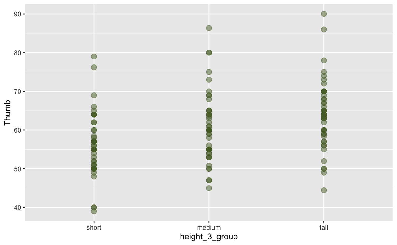
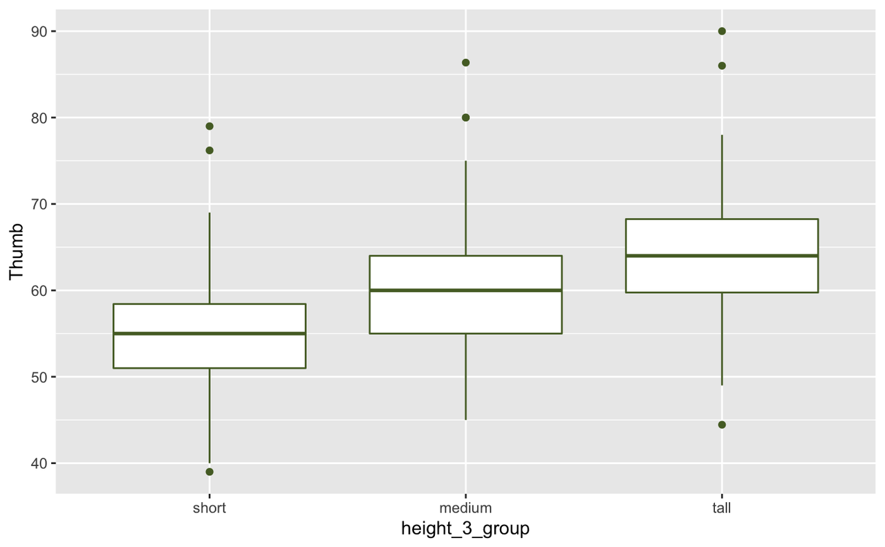
Looking at these two boxplots, we have an intuition that the three-group version of Height explains more variation in thumb length than does the two-group version. Although there is still a lot of variation within each group in the three-group version, the within-group variation appears smaller in the three-group than in the two-group model. Or, to put it another way, there is less variation left over after taking out the variation due to height.