5.4 Fitting the Empty Model
The simple model we have started with—using the mean to model the distribution of a quantitative variable—is sometimes called the empty model or null model. Note that it’s empty because it doesn’t have any explanatory variables in it yet. Our empty model does not explain any variation; it merely reveals the variation in the outcome variable that could be explained. If the mean is our model, then fitting the model to data simply means calculating the mean of the distribution.
Let’s think this through in the context of students’ thumb lengths. We will use a tiny data set, which we’ve put in a data frame called TinyFingers.
TinyFingers StudentID Thumb
1 1 56
2 2 60
3 3 61
4 4 63
5 5 64
6 6 68The whole data set is just six observations. Make a histogram of the distribution of six thumb lengths (Thumb). Add in a blue line to show where the mean is.
require(coursekata)

TinyFingers <- data.frame(
    StudentID = 1:6,
    Thumb = c(56, 60, 61, 63, 64, 68)
)
# modify this to save favstats for Thumb length
tinythumb_stats <-

# modify this to draw a vline representing the mean in "blue"
gf_histogram(~Thumb, data = TinyFingers) %>%
    gf_vline()
tinythumb_stats <- favstats(~Thumb, data = TinyFingers)
gf_histogram(~Thumb, data = TinyFingers) %>%
    gf_vline(xintercept = ~mean, color = "blue", data = tinythumb_stats)
ex() %>% {
    check_object(., "tinythumb_stats") %>%
        check_equal()

    check_function(., "gf_histogram") %>%
        check_result() %>%
        check_equal()

    check_or(.,
        check_function(., "gf_vline") %>%
            check_result() %>%
            check_equal(),
        override_solution(., "tinythumb_stats <- favstats(~Thumb, data = TinyFingers); gf_histogram(~Thumb, data = TinyFingers) %>% gf_vline(xintercept = ~tinythumb_stats$mean, color = 'blue')") %>%
            check_function(., "gf_vline") %>%
                check_result() %>%
                check_equal()
    )
}
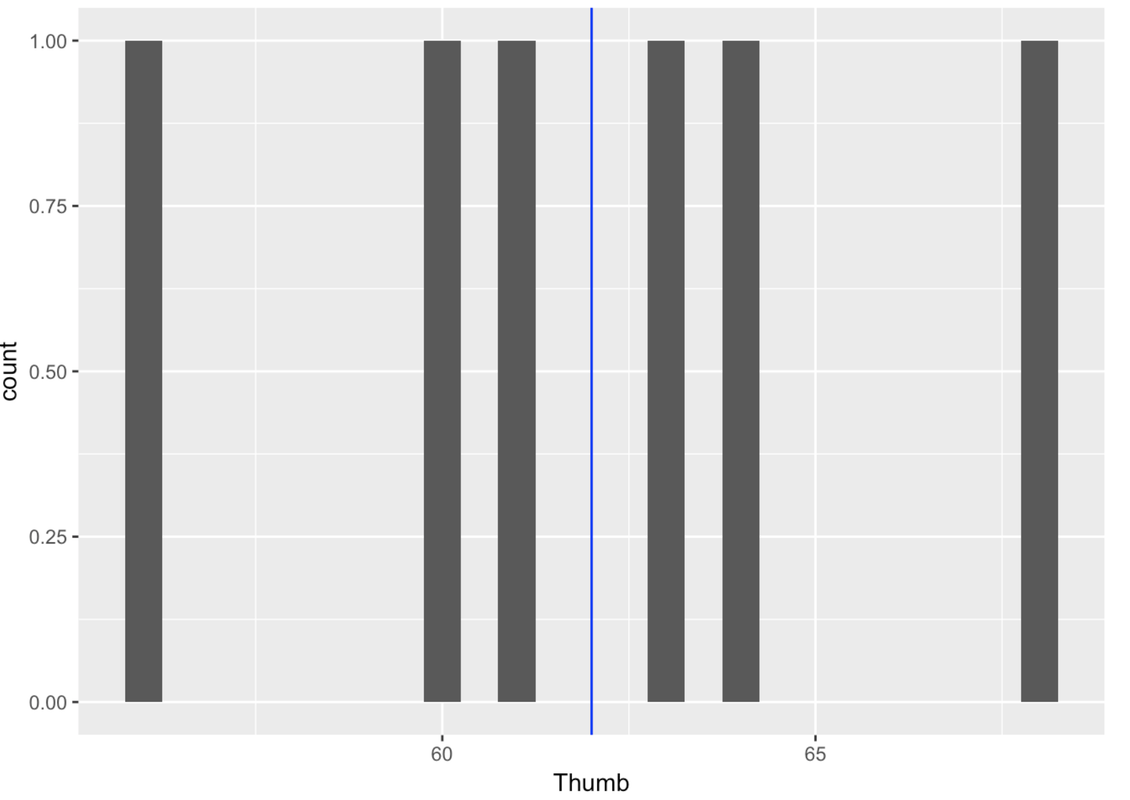
It’s easy to fit the empty model—it’s just the mean (62 in this case). But later you will learn to fit more complex models to your data. We are going to teach you a way of fitting models in R that you can use now for fitting the empty model, but that will also work later for fitting more complex models.
The R function we are going to use is lm(), which stands for “linear model.” (We’ll say more about why it’s called that in a later chapter.) Here’s the code we use to fit the empty model, followed by the output.
lm(Thumb ~ NULL, data = TinyFingers)Call:
lm(formula = Thumb ~ NULL, data = TinyFingers)
Coefficients:
(Intercept)
62Although the output seems a little strange, with words like “Coefficients” and “Intercept,” it does give you back the mean of the distribution (62), as expected. Thus, this function finds the best-fitting number for our model. The word “NULL” is another word for “empty” (as in “empty model.”)
It will be helpful to save the results of this model fit in an R object. Here’s code that uses lm() to fit the empty model, then saves the results in an R object called Tiny_empty_model:
Tiny_empty_model <- lm(Thumb ~ NULL, data = TinyFingers)If you want to see what the model estimates are after running this code, you can just type the name of the object where you saved the model:
Tiny_empty_modelCall:
lm(formula = Thumb ~ NULL, data = TinyFingers)
Coefficients:
(Intercept)
62We seem to be making a big deal about having calculated the mean of six numbers! But trust us, it will make more sense once you see where we go with it. One point is worth making now, however. Remember, the goal of statistics is to understand the DGP. The mean of the data distribution gives us our best estimate of the mean of the population that results from the DGP.
It may not be a very good estimate—after all, it is only based on a small amount of data—but it’s the best one we can come up with based on the available data. It also is an unbiased estimate, meaning that it is just as likely to be too high as it is too low.
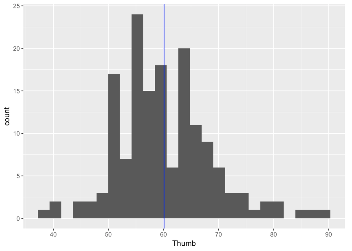
Now that you have fit the empty model to the tiny set of data, use lm() to fit the empty model to our full data set, Fingers.
Modify the code below to create a histogram of Thumb; draw a vertical line where the mean is; fit the empty model; and save the model to an R object called empty_model.
require(coursekata)
# modify this to fit the empty model of Thumb
empty_model <-

# this prints the best-fitting number
empty_model

# save the favstats for Thumb (this is helpful for drawing a line)
Thumb_stats <-

# make a histogram of Thumb and draw the line for the mean
gf_histogram() %>% gf_vline(xintercept = )
# modify this to fit the empty model of Thumb
empty_model <- lm(Thumb ~ NULL, data = Fingers)

# this prints the best-fitting number
empty_model

# save the favstats for Thumb (this is helpful for drawing a line)
Thumb_stats <- favstats(~Thumb, data = Fingers)

# make a histogram of Thumb and draw the line for the mean
gf_histogram(~Thumb, data = Fingers) %>%
    gf_vline(xintercept = ~mean, data = Thumb_stats)
ex() %>% {
    check_object(., "empty_model") %>% check_equal()
    check_object(., "Thumb_stats") %>% check_equal()
    check_function(., "gf_histogram") %>% {
        check_arg(., "object") %>% check_equal()
        check_arg(., "data") %>% check_equal()
    }
    check_function(., "gf_vline") %>% {
        check_arg(., "xintercept") %>% check_equal()
        check_arg(., "data") %>% check_equal()
    }
}
Call:
lm(formula = Thumb ~ NULL, data = Fingers)

Coefficients:
(Intercept)
       60.1
A common mistake when trying to add a line with data saved from favstats is to use the wrong data frame. The mean and median and other statistics are saved in the Thumb_stats data frame - not in the Fingers data frame!
In a single function, the data frame needs to actually contain the variable you are trying to use. The gf_histogram function uses the Thumb variable which is in the Fingers data frame. But you can chain on a different function that uses a totally different data frame. That’s why we can chain on the gf_vline function that uses the mean (which is a variable) in the Thumb_stats data frame.