5.5 Generating Predictions From the Empty Model
We have just made the point that the mean of the sample distribution is our best, unbiased estimate of the mean of the population. For this reason, we use the mean as our model for the population. And, if we want to predict what the next randomly sampled observation might be, without any other information, we would use the mean.
In data analysis, we also use the word “predict” in another sense and for another purpose. Using our tiny data set, we found the mean thumb length to be 62 mm. So, if we were predicting what the seventh observation might be, we’d go with 62 mm. But if we take the mean and look backwards at the data we have already collected, we could also generate a “predicted” thumb length for each of the data points we already have. This prediction answers the question: what would our model have predicted this thumb length to be if we hadn’t collected the data?
There’s an R function that will actually do this for you. Here’s how we can use it to generate the predicted thumb lengths for each of the six students in the tiny data set. Remember, we already fit the model and saved the results in Tiny_empty_model:
predict(Tiny_empty_model) 1 2 3 4 5 6
62 62 62 62 62 62Now, why would we want to create predicted thumb lengths for these six students when we already know their actual thumb lengths? We will go into this a lot more in the next chapter, but for now, the reason is so we can get a sense of how far each of our data points are from the prediction that our model would have made. In other words, it gives us a rough idea of how well our model fits our current data.
In order to use these predicted scores as a way of seeing how much error there is, we first need to save the prediction for each student in the data set. When there is only one prediction for everyone, as with the empty model, and when there are only six data points, as in our tiny data set, it seems like overkill to save the predictions.
But later you will see how useful it is to save the individual predicted scores. For example, if we save the predicted score for each student in a new variable called Predicted, we can then subtract each student’s actual thumb length from their predicted thumb length, resulting in a deviation from the prediction.
Use the function predict() and save the predicted thumb lengths for each of the six students as a new variable in the TinyFingers data set. Then, print the new contents of TinyFingers.
require(coursekata)

TinyFingers <- data.frame(
    StudentID = 1:6,
    Thumb = c(56, 60, 61, 63, 64, 68)
)
Tiny_empty_model <- lm(Thumb ~ NULL, data = TinyFingers)
# modify this to save the predictions from the Tiny_empty_model
TinyFingers$Predicted <-

# this prints TinyFingers
TinyFingers
TinyFingers$Predicted <- predict(Tiny_empty_model)
TinyFingers
ex() %>% check_object("TinyFingers") %>%
check_column("Predicted") %>% check_equal() StudentID Thumb Predicted
1 1 56 62
2 2 60 62
3 3 61 62
4 4 63 62
5 5 64 62
6 6 68 62Thinking About Error
We have developed the idea of the mean being the simplest (or empty) model of the distribution of a quantitative variable. If we connect this idea to our general formulation DATA = MODEL + ERROR, we can rewrite the statement as:
DATA = MEAN + ERROR
If this is true, then we can calculate error in our data set by just shuffling this equation around to get the formula:
ERROR = DATA - MEAN
Using this formula, if someone has a thumb length larger than the mean (e.g., 68), then their error is a positive number (in this case, +6). If they have a thumb length lower than the mean (e.g., 61) then we can calculate their error as a negative number (e.g. -1).
We generally call this calculated error the residual, the difference between our model’s prediction and an actual observed score. The word residual should evoke the stuff that remains because the residual is the leftover quantity from our data once we take out the model.
To find these errors (or residuals) you can just subtract the mean from each data point. In R we could just run this code to get the residuals:
TinyFingers$Thumb - TinyFingers$Predicted[1] -6 -2 -1 1 2 6The numbers in the output indicate, for each student in the data frame, what their residual is after subtracting out the model (which is the mean in this case).
Modify the following code to save these residuals in a new variable in TinyFingers called Residual.
Modify the following to save these residuals as part of the TinyFingers data frame.
require(coursekata)

TinyFingers <- data.frame(
    StudentID = 1:6,
    Thumb = c(56, 60, 61, 63, 64, 68)
)
Tiny_empty_model <- lm(Thumb ~ NULL, data = TinyFingers)
TinyFingers <- TinyFingers %>% mutate(
    Predicted = predict(Tiny_empty_model)
)
# modify this to save the residuals from the Tiny_empty_model
TinyFingers$Residual <-

# this prints TinyFingers
TinyFingers
TinyFingers$Residual <- TinyFingers$Thumb - TinyFingers$Predicted
TinyFingers
ex() %>% check_object("TinyFingers") %>%
check_column("Residual") %>% check_equal() StudentID Thumb Predicted Residual
1 1 56 62 -6
2 2 60 62 -2
3 3 61 62 -1
4 4 63 62 1
5 5 64 62 2
6 6 68 62 6These residuals (or “leftovers”) are so important in modeling that there is an even easier way to get them in R. Again, we will use the results of our model fit, which we saved in the R object Tiny_empty_model:
resid(Tiny_empty_model) 1 2 3 4 5 6
-6 -2 -1 1 2 6Notice that we get the same numbers. But instead of specifying the data and the model’s predictions, we just tell R which model to get the residuals from.
Modify the following code to save the residuals that we get using the resid() function in the TinyFingers data frame. Give the resulting variable a new name: EasyResidual.
require(coursekata)

TinyFingers <- data.frame(
    StudentID = 1:6,
    Thumb = c(56, 60, 61, 63, 64, 68)
)
Tiny_empty_model <- lm(Thumb ~ NULL, data = TinyFingers)
TinyFingers <- TinyFingers %>% mutate(
    Predicted = predict(Tiny_empty_model)
)
# modify this to save the residuals from the Tiny_empty_model (calculate them the easy way)
TinyFingers$EasyResidual <-

# this prints TinyFingers
TinyFingers
TinyFingers$EasyResidual <- resid(Tiny_empty_model)
TinyFingers
ex() %>% check_object("TinyFingers") %>%
    check_column("EasyResidual") %>% check_equal()
success_msg("Fantastic work!") StudentID Thumb Predicted Residual EasyResidual
1 1 56 62 -6 -6
2 2 60 62 -2 -2
3 3 61 62 -1 -1
4 4 63 62 1 1
5 5 64 62 2 2
6 6 68 62 6 6Note that the variables Residual and EasyResidual are identical. This makes sense; you just used different methods to get the residuals.
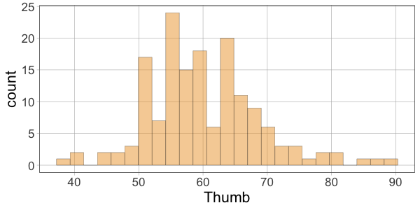
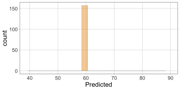
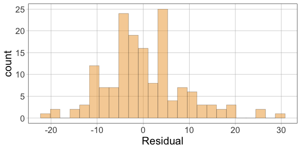
Here we’ve plotted histograms of the three variables: Thumb, Predicted, and Residual.
The distributions of the data and the residuals have the same shape. But the numbers on the x-axis differ across the two distributions. The distribution of Thumb is centered at the mean (62), whereas the distribution of Residual is centered at 0. Data that are smaller than the mean (such as a thumb length of 58) have negative residuals (-4) but data that are larger than the mean (such as 73) have positive residuals (11).
Print out the favstats() for Thumb and the Residual for the TinyFingers data frame.
require(coursekata)

TinyFingers <- data.frame(
    StudentID = 1:6,
    Thumb = c(56, 60, 61, 63, 64, 68)
)
Tiny_empty_model <- lm(Thumb ~ NULL, data = TinyFingers)
TinyFingers <- TinyFingers %>% mutate(
    Predicted = predict(Tiny_empty_model),
    Residual = resid(Tiny_empty_model)
)
# get the favstats for Thumb

# get the favstats for Residual

# if you decide to save them, make sure to print them out
favstats(~Thumb, data = TinyFingers)
favstats(~Residual, data = TinyFingers)
ex() %>% {
    check_output_expr(., "favstats(TinyFingers$Thumb)")
    check_output_expr(., "favstats(TinyFingers$Residual)")
}
success_msg("You're getting the hang of it!") min Q1 median Q3 max mean sd n missing
56 60.25 62 63.75 68 62 4.049691 6 0 min Q1 median Q3 max mean sd n missing
-6 -1.75 -1.421085e-14 1.75 6 -1.421085e-14 4.049691 6 0R will sometimes give you outputs like the value for the mean of the residuals: -1.421085e-14. The e-14 part indicates that this is a number very close to zero (the -14 meaning that that decimal point is shifted to the left 14 places)! Whenever you see this scientific notation with a large negative exponent after the “e”, you can just read it as “zero,” or pretty close to zero.
The residuals (or error) around the mean always sum to 0. Therefore, the mean of the errors will also always be 0, because 0 divided by n equals 0. (R will not always report the sum as exactly 0 because of computer hardware limitations but it will be close enough to 0.)
Now that you have looked in detail at the tiny set of data, explore the predictions and residuals from the empty_model fit earlier from the full set of Fingers data. Add them as new variables (Predicted and Residual) to the Fingers data frame.
require(coursekata)
# this code from before fits the empty model for Fingers
Empty.model <- lm(Thumb ~ NULL, data = Fingers)

# generate predictions from the Empty.model
Fingers$Predicted <-

# generate residuals from the Empty.model
Fingers$Residual <-

# this prints out 10 lines of Fingers
head(select(Fingers, Thumb, Predicted, Residual), 10)
Empty.model <- lm(Thumb ~ NULL, data = Fingers)
Fingers$Predicted <- predict(Empty.model)
Fingers$Residual <- resid(Empty.model)
head(select(Fingers, Thumb, Predicted, Residual), 10)
ex() %>% check_object("Fingers") %>% {
    check_column(., "Predicted")
    check_column(., "Residual")
} Thumb Predicted Residual
1 66.00 60.10366 5.8963376
2 64.00 60.10366 3.8963376
3 56.00 60.10366 -4.1036624
4 58.42 60.10366 -1.6836624
5 74.00 60.10366 13.8963376
6 60.00 60.10366 -0.1036624
7 70.00 60.10366 9.8963376
8 55.00 60.10366 -5.1036624
9 60.00 60.10366 -0.1036624
10 52.00 60.10366 -8.1036624Then make histograms of the variables Thumb, Predicted, and Residual. Which two histograms will have a similar shape?
require(coursekata)

empty_model <- lm(Thumb ~ NULL, data = Fingers)
Fingers <- supernova::Fingers %>% mutate(
    Predicted = predict(empty_model),
    Residual =  resid(empty_model)
)
# make a histogram for Thumb
gf_histogram(  )

# make a histogram for Predicted
# leave the gf_lims() part -- it makes the graph easier to read
gf_histogram(  ) %>%
  gf_lims(x = range(Fingers$Thumb))

# make a histogram for Residual
gf_histogram(  )
# make a histogram for Thumb
gf_histogram(~Thumb, data = Fingers)

# make a histogram for Predicted
# leave the gf_lims() part -- it makes the graph easier to read
gf_histogram(~Predicted, data = Fingers) %>%
  gf_lims(x = range(Fingers$Thumb))

# make a histogram for Residual
gf_histogram(~Residual, data = Fingers)
ex() %>% {
    check_function(., "gf_histogram", index = 1) %>% check_result() %>% check_equal()
    check_function(., "gf_histogram", index = 2) %>% check_result() %>% check_equal()
    check_function(., "gf_histogram", index = 3) %>% check_result() %>% check_equal()
}