8.2 Fitting a Regression Model

Using lm() to Fit the Height Model to TinyFingers

Now you can begin to see the power you’ve been granted by the General Linear Model fitting—or estimating the parameters—of the regression model, is accomplished the same way as estimating the parameters of the grouping model. It’s all done using the lm() function in R.

The lm() function is smart enough to know that if the explanatory variable is quantitative, the model to estimate is the regression model. If the explanatory variable is categorical (e.g., defined as a factor in R), lm() will fit a group model.

Modify the code below to fit the regression model using Height as the explanatory variable to predict Thumb length in the TinyFingers data.

Call:
lm(formula = Thumb ~ Height, data = TinyFingers)

Coefficients:
(Intercept)       Height  
    -3.1611       0.9848

Fitting a Regression Model By Accident When You Don’t Want One

Although R is pretty smart about knowing which model to fit, it won’t always do the right thing. If you code the grouping variable with the character strings “short” and “tall,” R will make the right decision because it knows the variable must be categorical. But if you code a grouping variable as 1 and 2, and you forget to make it a factor, R may get confused and fit the model as though the explanatory variable is quantitative.

For example, we’ve added a new variable to our TinyFingers data called GroupNum. Here is what the data look like.

  Thumb Height Height2Group GroupNum
1    56     62        Short        1
2    60     66        Short        1
3    61     67         Tall        2
4    63     63        Short        1
5    64     68         Tall        2
6    68     71         Tall        2

If you take a look at the variables Height2Group and GroupNum, they have the same information. Students 1, 2, and 4 are in one group and students 3, 5, and 6 are in another group. If we fit a model with Height2Group (and called it the Height2Group.model) or GroupNum (and called it the GroupNum.model), we would expect the same estimates. Let’s try it.

Call:
lm(formula = Thumb ~ Height2Group, data = TinyFingers)

Coefficients:
       (Intercept)  Height2GroupTall  
            59.667             4.667

Call:
lm(formula = Thumb ~ GroupNum, data = TinyFingers)

Coefficients:
(Intercept)     GroupNum  
     55.000        4.667

Because Height2Group is a factor (i.e., a categorical variable), lm() fits a group model. But for GroupNum, lm() thinks the 1 or 2 coding refers to a quantitative variable because we did not tell R that it was a factor. So it fits a regression line instead of a group model. If it does that, the meaning of the estimates will not be what you expect for the group model.

The slope will be accurate, because it will tell you the increment in thumb length between people coded as 2 versus those coded as 1. But the \(b_{0}\) estimate will be the y-intercept—that is, the predicted thumb length when \(X_{i}\) equals 0. This makes no sense when there are only two groups and they are coded 1 and 2. This is an accidental regression model.

Try it here by recoding GroupNum as 0 and 1. See if the results fit your expectations.

Fitting the Height Model to the Full Fingers Data Set

Now that you have looked in detail at the tiny set of data, fit the height model to the full Fingers data frame, and save the model in an R object called Height.model.

Call:
lm(formula = Thumb ~ Height, data = Fingers)

Coefficients:
(Intercept)       Height  
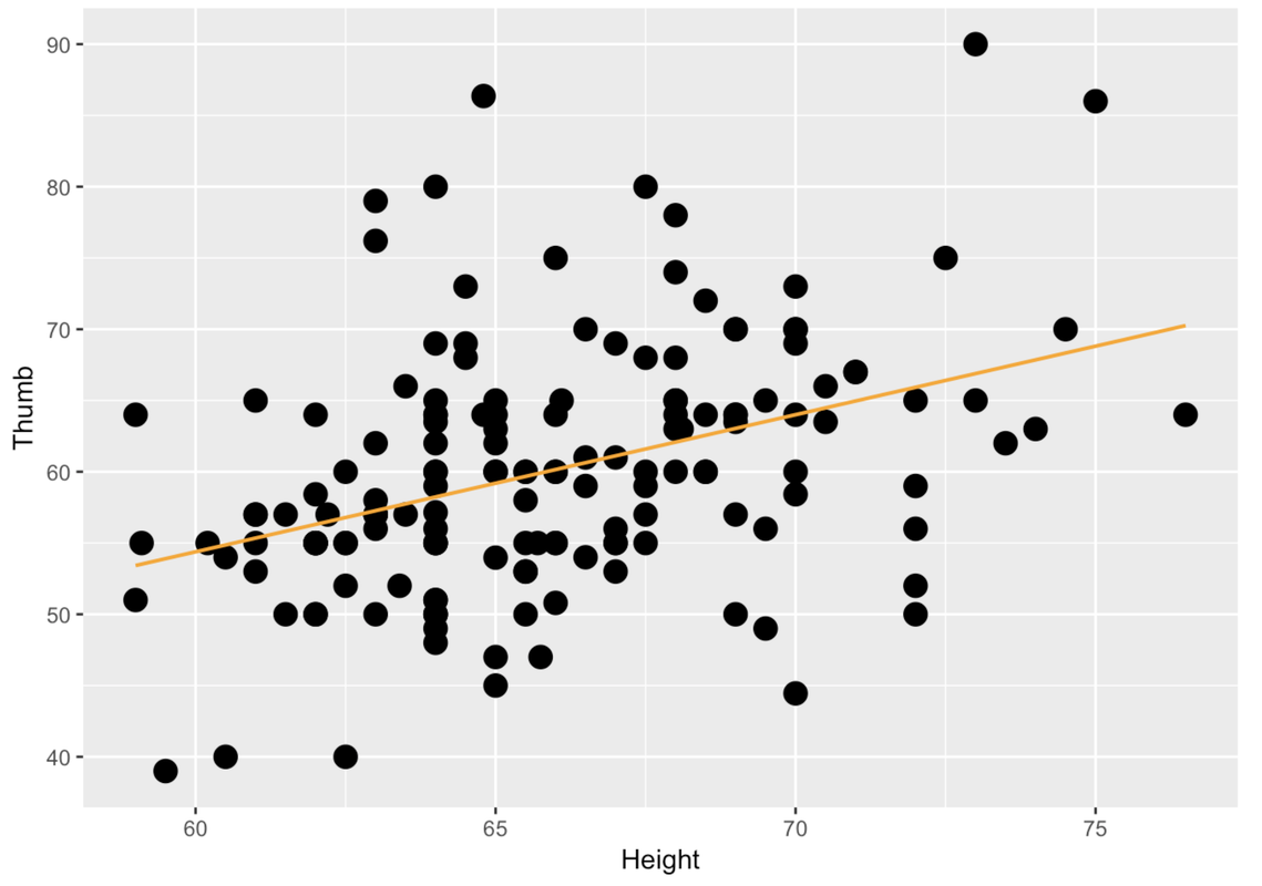
    -3.3295       0.9619

Here is the code to make a scatter plot to show the relationship between Height (on the x-axis) and Thumb (on the y-axis) for TinyFingers. Note that the code also overlays the best-fitting regression line on the scatter plot. Edit the code to make this scatter plot for the full Fingers data set.