Chapter 10 - Confidence Intervals and their Uses

10.0 Confidence Intervals: Estimating the Error in an Estimate

In the previous chapter we developed the concept of sampling distribution. When we conduct a study we collect a sample of data, randomly sampled from some population. Based on the sample, we calculate statistics such as the mean of a quantitative variable. We use this mean as an estimate of the population mean.

Sampling distributions help us to put this sample mean — the one we can calculate — into the context of other means that could have resulted had we chosen different random samples. If the sampling distribution is spread out, then we know that our particular estimate could be off by quite a bit. But if the sampling distribution is narrow, we can be sure that our estimate is fairly close to the true population mean.

Confidence intervals let us build on this logic to quantify how far off our estimate might be, based on the characteristics of sampling distributions. Instead of just a qualitative statement of how much fluctuation there might be in our estimate, confidence intervals let us say things like: “Our estimate of the true mean is 60.1 mm. But we can say with 95% confidence that the true mean is somewhere between 58.72 and 61.52.”

Note: this does not mean that the probability of the true mean being between 58.72 and 61.52 is .95. Technically, what it means is that the true mean will be contained within the confidence interval for 95% of random samples that you could draw. This is not an easy distinction to understand, so don’t worry if it seems obtuse. Just keep it in mind as you go.

The Basic Idea Behind Confidence Intervals

The basic logic behind confidence intervals was developed in the previous chapter. But it’s a hard concept to understand, so it’s worth reviewing it again.

Let’s start with the idea that the mean we observe in our sample of data is just one of many possible means that could have resulted had we chosen different random samples. We must conceptualize these many possible means as being random samples of a particular size from a sampling distribution of means.

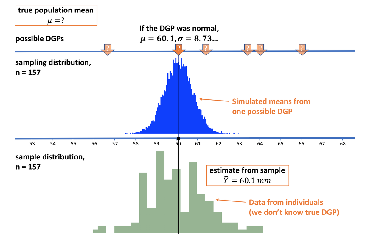
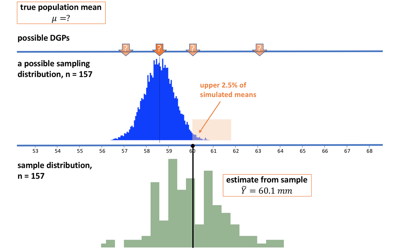
In the picture above, we see our sample represented on the bottom, in green. Our estimate of the population mean, based on our sample, is 60.1 mm (represented by the black dot and line). At the very top of the figure, you see that we actually do not know what the population mean (\(\mu\)) is.

Nevertheless, we are going to use our “If…” thinking and assume, for a moment, one possible DGP. We will assume it is normal, has a mean of 60.1 mm and a standard deviation of 8.73. Again, this is just one possible DGP out of an infinite number of possibilities.

Above the number line, measured off in the units of the outcome variable (thumb length in mm), we have pictured the sampling distribution of means of samples of n=157 generated by this one possible DGP.

We can see that our observed mean is a possible mean from such a DGP, which makes sense: we chose this guess of the DGP to be centered exactly at the mean we observed in our sample. But it is important to recognize that our observed mean could easily have been generated by other possible DGPs as well.

We created this particular sampling distribution by simulation, but we could have used the Central Limit Theorem if we wanted. However we create it, the sampling distribution is a theoretical model; it doesn’t really exist, we just make it up to help us think about the mean we calculated based on our sample.

The shape of the sampling distribution of means is normal (we know this will be true based on the Central Limit Theorem and simulations), and its spread is based on our estimate of the population standard deviation. The standard deviation of the sampling distribution is called the standard error. We know, both from simulations and from the Central Limit Theorem, that the standard error will get lower as the sample size (n) gets larger. And, importantly, the spread of the sampling distribution will always be less than the spread of the population distribution (unless n=1, in which case the sampling distribution would look identical to the population distribution).

We know that the true sampling distribution will have the same mean as the population (\(\mu\)). But what we don’t know is the mean of the population. So, although we pictured the sampling distribution, above, centered on our sample mean of 60.1 mm, we can be virtually certain that this is wrong! It might be true (slight chance), or it might be close (slightly higher chance). But it is almost certainly wrong.

The sample mean is the best estimate we have of the population mean, but it is only an estimate. The true population mean is probably different from our estimate. The question is: how different? How low could the true population mean be? Or how high? This is what we want to find out.

We can represent this question by moving the hypothetical population mean and its corresponding sampling distribution around on the number line. We won’t change the shape or spread of the sampling distribution, but we must consider a range of possible DGPs that could have generated these imaginary samples.

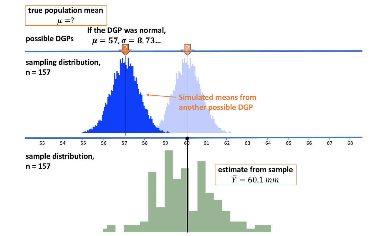
Let’s imagine a different possible DGP: one with a mean of 57. If the true mean of the DGP were 57, the imaginary sampling distribution would be generated more to the left, as pictured above, centered over a mean of 57 mm.

How likely is it that our sample, and its sample mean, could have been drawn from this new sampling distribution with \(\mu\) of 57? It would appear very unlikely. None of the simulated sample means (the dark blue simulated histogram) are anywhere near as high as the 60.1 mm we observed.

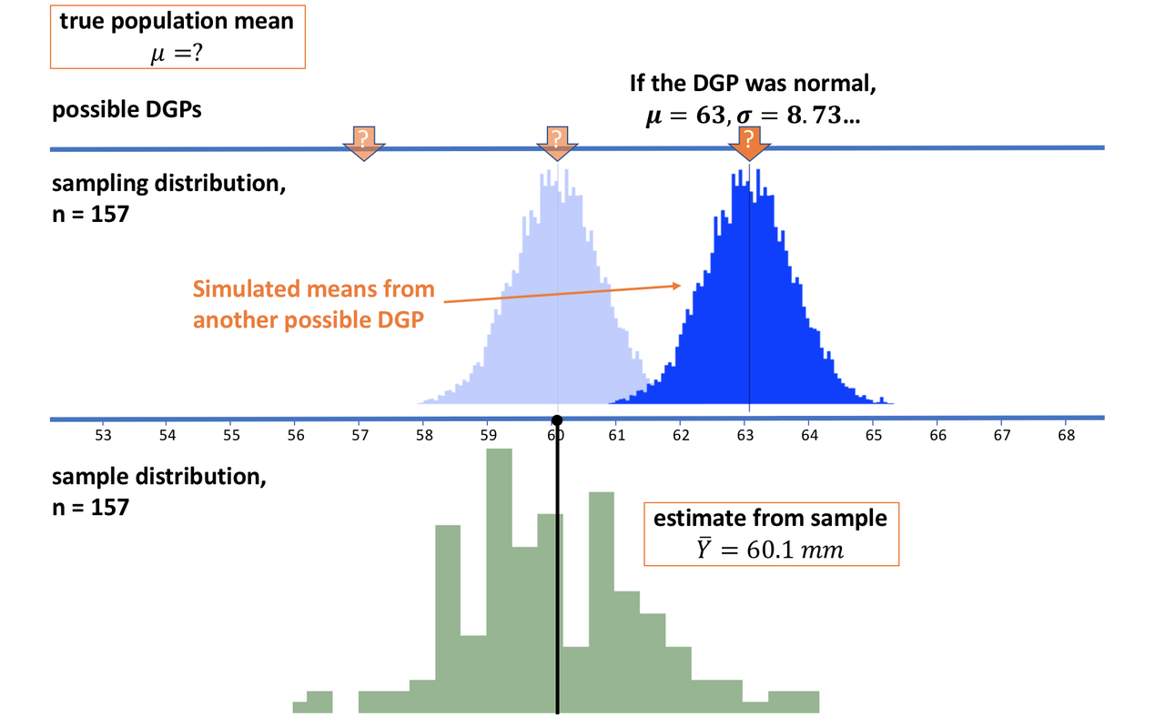
If we slide the hypothesized population and sampling distribution the other way, to the right, we can draw a similar conclusion. It is very unlikely that our sample was drawn from a sampling distribution (and thus a population) with a mean as high as 63. As a start, then, we can be pretty sure that the true population mean is somewhere between 57 and 63. Let’s now see if we can narrow that down even further.

Defining Likely: Putting the “95” into the 95% Confidence Interval

We have established that it is unlikely that the sample mean we observed came from a population with a true mean as high as 63. In fact, it looks very unlikely. But let’s now slide our imagined sampling distribution back to the left, until the mean of our sample lines up exactly with the point below which 2.5% of the simulated sample means in the sampling distribution fall (see picture below).

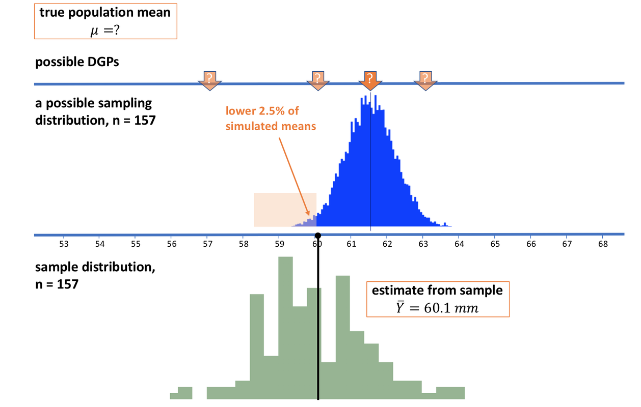
The simulated means in the light orange region would only occur in 2.5% of random samples of n=157 generated by this DGP. We decide, just by convention, to consider anything with a less than 2.5% chance of occurring “unlikely.” We slide our sampling distribution around until our observed sample mean of 60.1 falls right at this boundary. We will consider our observed mean in the “likely” category, but any sample with a lower mean than the one we observed we will consider unlikely.

We haven’t yet figured out what the mean of the blue sampling distribution is, except that we know it is the same as the assumed mean of the DGP. Whatever it is, though, (and from the picture it looks to be somewhere between 61 and 62 mm) our sample would be one of the lowest means that are still considered “likely” under this sampling distribution.

We’ll call this unknown population mean the upper bound for now. If you generated a sampling distribution from a population mean any higher than this upper bound, then our observed sample mean would then fall into the “unlikely” area. Thus, there is a less than 2.5% chance that our sample mean came from a population with a mean higher than the upper bound.

If we repeat this move in the other direction, we can find a sampling distribution under which our observed sample mean would be one of the highest “likely” means. In the sampling distribution above, only 2.5% of the simulated sample means are higher than the mean we observed. We’ll call the mean of the population that generated these samples the lower bound.

We can get a sense of this lower bound by looking at the mean of the sampling distribution at this point (which appears to be between 58 and 59 mm). If the population mean were any lower than our lower bound, our sample mean would have a 2.5% chance or less of being drawn.

Putting this all together, if our sample mean has only a 2.5% chance of being from a population lower than our lower bound, and a 2.5% chance of being from a population higher than our higher bound, it follows that we can be 95% confident that the true population mean is somewhere between the two boundaries. This interval is the 95% confidence interval.

Finding the Margin of Error

Now that we see the logic, all that remains is to find the exact distance between the boundaries of the “unlikely” areas for the lower and upper sampling distributions, and the means of those two distributions (which represent the lower and upper possible values for the population mean). We refer to this distance as the margin of error (sometimes you may see it referred to as the “critical distance”). The units of the margin of error should be in mm, the scale of our outcome variable.

Note that a distance is always positive. So even though we talk about a margin of error as plus or minus a certain distance from the mean, the distance itself is positive. Whether you walk forwards or backwards, the distance you walk is still positive.

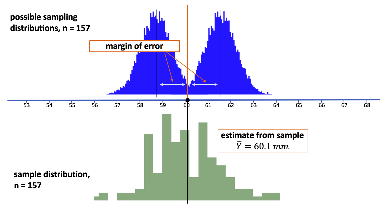
As you can see in the picture, because we have lined up the boundaries of the 2.5% unlikely areas right on the sample mean (60.1 mm), we can simply add the margin of error to our sample mean to get the upper bound, and subtract the margin of error from the sample mean to get the lower bound of the 95% confidence interval.

Let’s see if we can explain a little more about why this works. First of all, it’s important to remember that when we slide these sampling distributions up and down, we are not changing their shape (normal) or their standard deviation. What we are changing is the assumed mean of the population that generated the sampling distributions (which gets reflected in the mean of the sampling distribution).

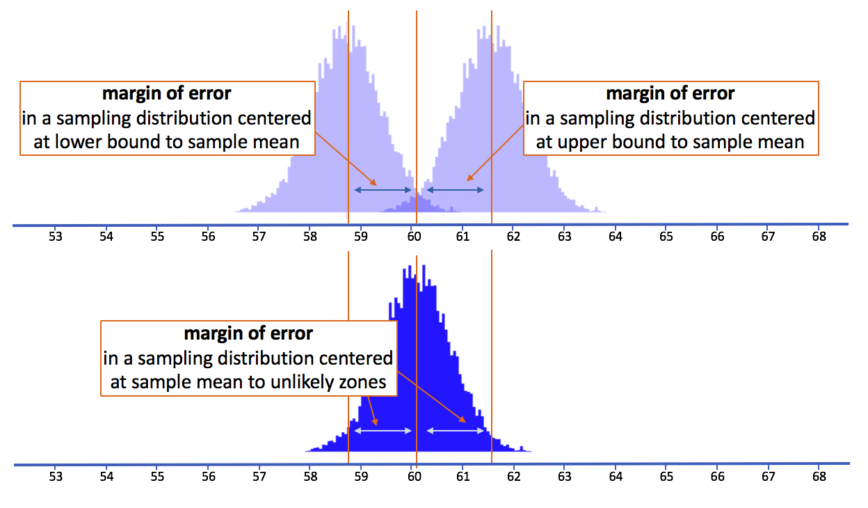
In this picture we have depicted three sampling distributions. The one on the bottom (in darker blue) is centered on our sample mean. The two on the top (in lighter blue) are centered on the upper and lower bounds which correspond perfectly to the cutoff points that demarcate the middle 95% of the sampling distribution centered on the sample mean.

Notice that the light blue margin of error in the dark blue sampling distribution is the same length as the darker blue margin of error in the light blue sampling distributions. That is, the distance from the mean of the dark blue sampling distribution to the lower 2.5% of its means is the same as the distance from the mean of the light blue lower bound sampling distribution to the upper 2.5% of its means.

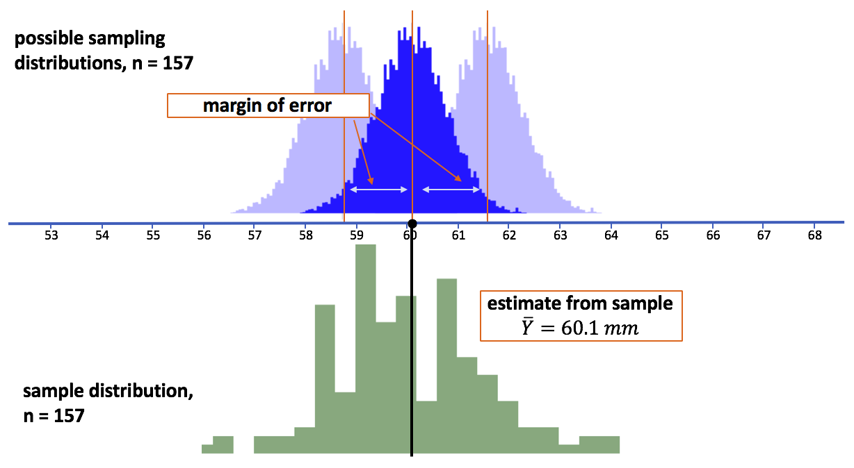
In this picture (above) we have just put all three of these sampling distributions on top of each other to drive home the convenient fact that the margin of error is the same regardless of where we center the mean of the sampling distribution.

Because we are using the same sampling distribution (meaning it has the same shape and standard error), just sliding it back and forth, we can calculate the margin of error by centering the simulated sampling distribution on our observed sample mean, and then finding the distance from the sample mean to the upper and lower boundary points.

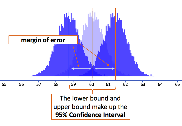
The two cutoff points in the sampling distribution centered at the sample mean (2.5% in the lower tail and 2.5% in the upper tail) will be exactly at the lower and upper boundaries of possible values for the population mean (see picture above).

Thus, to calculate the 95% confidence interval we can just look at the cutoff points in the sampling distribution centered at the mean. Another method of finding confidence intervals would be to take the mean of our sample, plus or minus the margin of error. The actual meaning of the 95% confidence interval, however, is this: the lower and upper bounds represent the possible population means below and above which it would be unlikely to have generated the sample mean that we observed.