9.4 Simulating Samples to Create a Sampling Distribution

Simulating Some Samples of Thumb Lengths

Now let’s extend our simulation to illustrate the concept of a sampling distribution. We will assume the same things about the DGP as in the previous simulation: normal distribution with a \(\mu\) of 60.1 and a \(\sigma\) of 8.73.

Let’s start by generating a single sample of n=157 thumb lengths from the same assumed DGP. We could use this code:

rnorm(157, mean = 60.1, sd = 8.73)

But we will often choose to write this code:

rnorm(157, mean = Thumb.stats$mean, sd = Thumb.stats$sd)

Mostly we use the latter because we find it annoying to have to remember what the numbers are. Also, an added benefit is that when we just use Thumb.stats, we don’t have to worry about rounding our numbers; R will just use the super-long decimal because computers are good at remembering all the digits.

Why, you may ask, are you simulating a sample of 157 thumb lengths? The reason is that 157 is the exact size of the sample we collected for our study. Simulation of samples of n=157 lets us explore the kind of variation we might see among random samples of 157 thumbs.

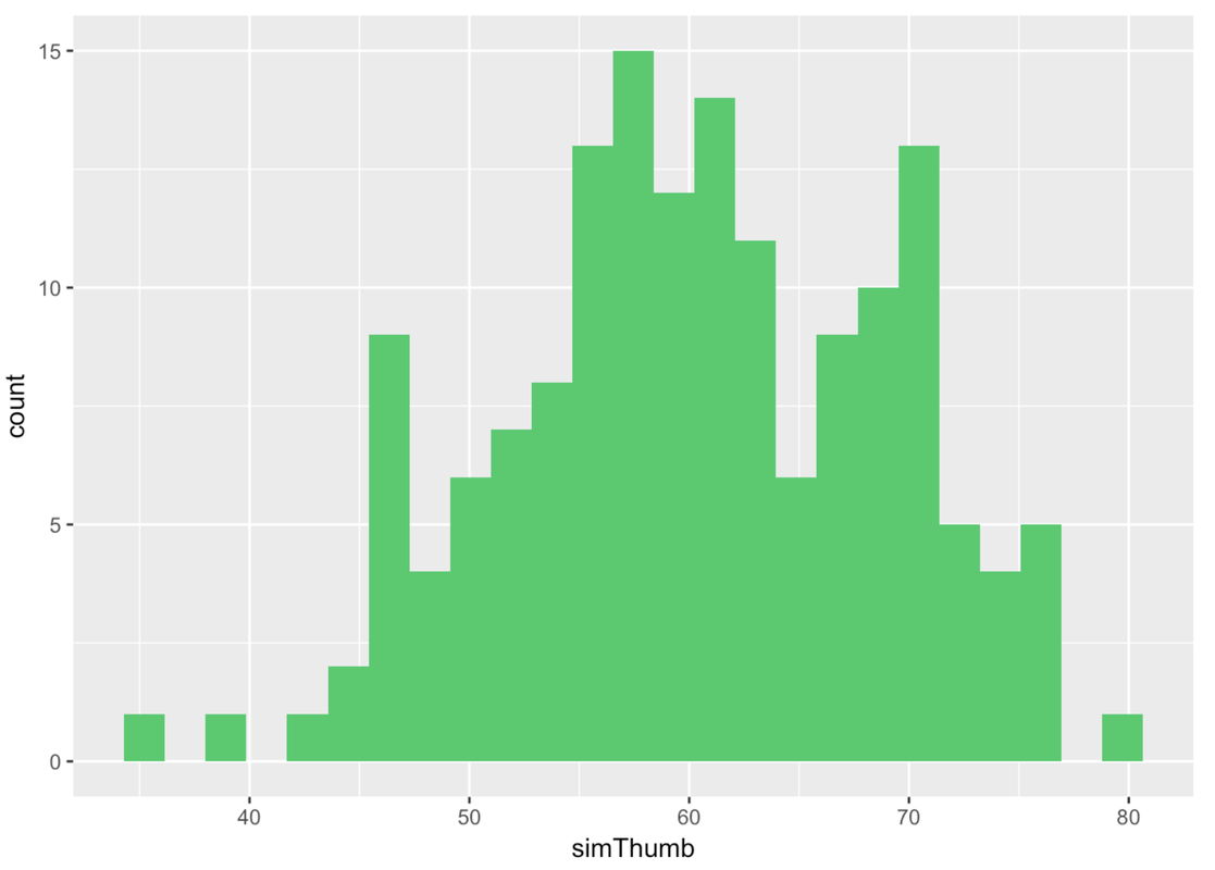
So we’ll run this code rnorm(157, mean = Thumb.stats$mean, sd = Thumb.stats$sd) and put it into a data frame and all that in order to plot the simulated thumb lengths in a histogram. We’ll put simulated Thumb data in green (specifically “springgreen3”) so you don’t confuse it for real data.

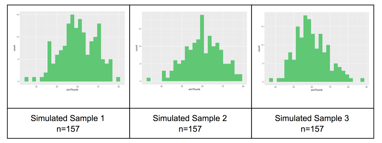
Let’s generate two more samples, and look at all three simulated samples next to each other.

Now look at the histogram below. This is our actual distribution (again) of the thumb lengths produced by our sample of 157 students.

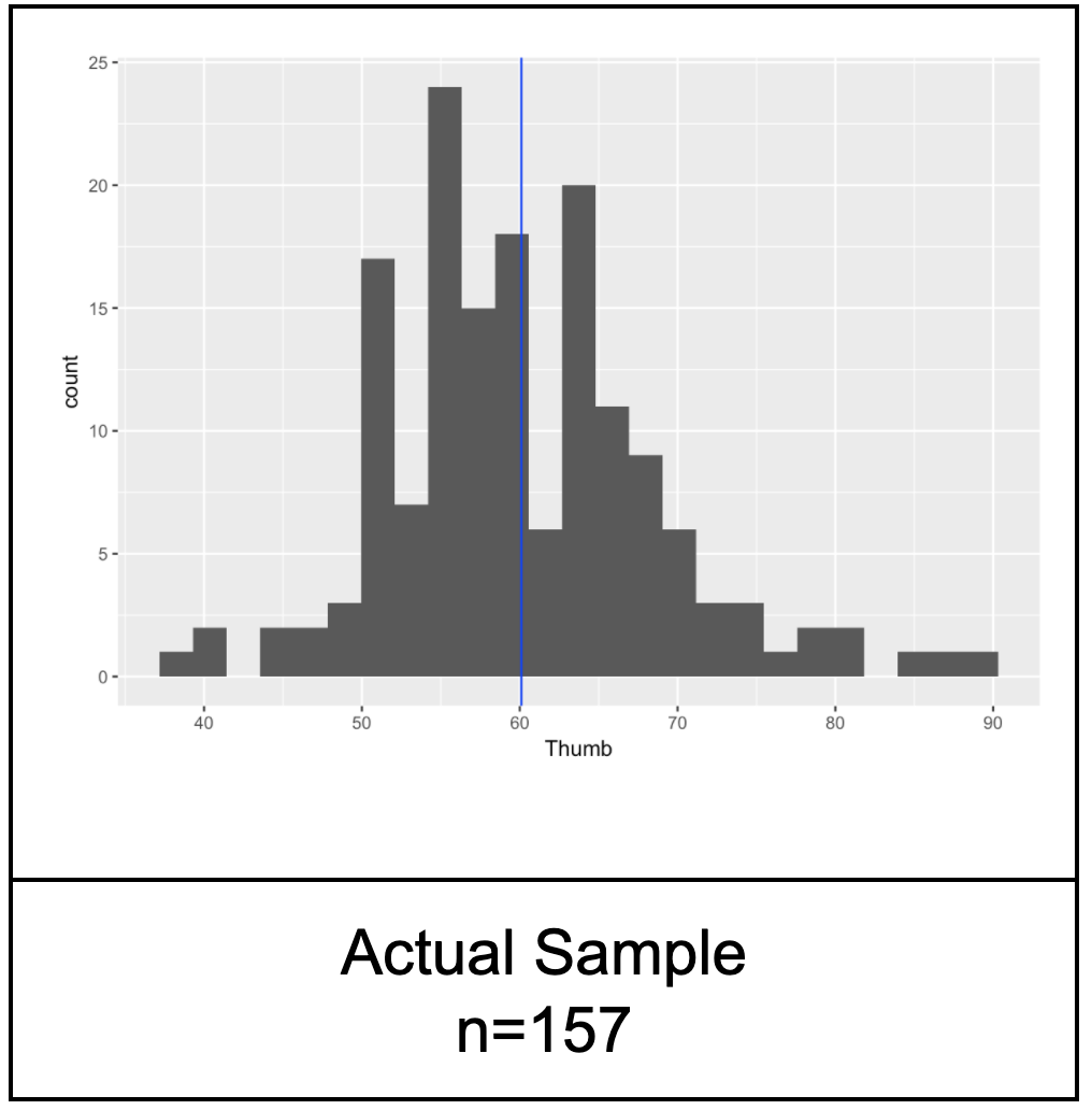
Compare the actual distribution with the three simulated sample distributions. Notice that our real sample basically doesn’t look that different from the simulated samples. The simulated samples all vary to some degree and our sample could blend in with them.

Already, just by looking at some simulated samples of the same size we studied, we can get a sense of what our data could have looked like if we had selected a different sample. It certainly seems reasonable, based on just looking at histograms, that our sample could have been generated with the DGP we assumed for our simulations: a normal distribution with a mean of 60.1 and a standard deviation of 8.73.

Simulating a Sampling Distribution of Mean Thumb Lengths

Up to this point we have generated some samples of n=157 and examined their distributions visually. To construct a sampling distribution, however, we need to compute a sample statistic such as the mean, and do it for a large number of simulated samples.

We learned before how to calculate the mean of 24 randomly-generated die rolls.

mean(resample(1:6, 24))

Then we learned how to generate individual scores from a hypothetical normal distribution.

rnorm(1, mean = Thumb.stats$mean, sd = Thumb.stats$sd)

Let’s try to put these two ideas together. Modify this code to get the mean of 157 randomly-generated scores from our assumed DGP.

[1] 60.86912

It is important to note that this 60.86912 is not an individual thumb length, but the average of 157 randomly-generated thumb lengths.

Now let’s generate some more samples of n=157. Modify the code below using the do() function to generate 20 samples of n=157.

       mean
1  60.95947
2  60.90133
3  59.96278
4  60.65892
5  60.76355
6  60.78775
7  60.57710
8  60.33422
9  60.61046
10 59.83752
11 60.73043
12 60.36514
13 60.88077
14 60.82883
15 58.86428
16 59.44147
17 59.41052
18 60.67863
19 59.06284
20 59.23941

Notice that the individual thumb lengths have some extreme thumbs like 74 mm and 40 mm. But the means of samples of n=157 are less extreme.

In the previous section, we generated 1,000 individual thumb lengths to create a simulated population. Now let’s create a simulated sampling distribution. Modify the code we provided to calculate 1,000 means from samples of n=157 from the same hypothesized DGP as above. We’ll save the resulting 1,000 sample means in a data frame called SDoM, short for Sampling Distribution of Means. Then print out the first six rows of SDoM.

      mean
1 60.95947
2 60.90133
3 59.96278
4 59.65892
5 60.76355
6 60.78775

Use the code window below to make a histogram of the variable mean in SDoM. Also calculate the favstats() for this distribution of means.

      min       Q1   median       Q3      max     mean        sd     n missing
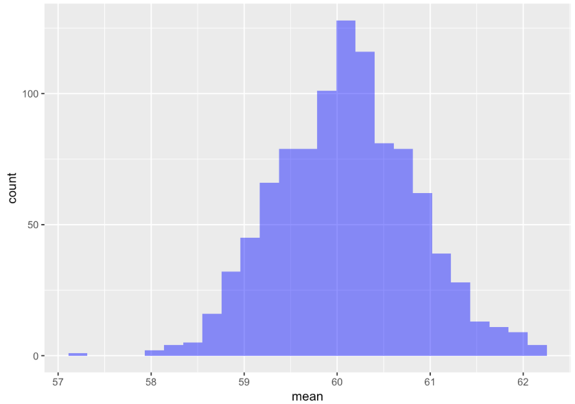
 57.19678 59.61451 60.08462 60.56124 62.70251 60.09452 0.7374960  1000       0

The resulting distribution is not a distribution of individual thumb lengths—it’s a distribution of means of samples of n=157. We can see from the histogram that even though we know that the population mean is 60.1, it’s still possible that a randomly selected sample of n=157 could have a mean as large as 62 mm or as small as 58 mm. Most of the means, however, seem to cluster around 60.1, the mean of the population from which the samples were drawn. Your SDoM (and resulting favstats) should look similar to what we got, but it won’t look exactly the same because each random simulation will vary a little.

Here the two simulated distributions are shown side-by-side: the population (on the left) and the sampling distribution (on the right). On the left, each data point represents the thumb length of an individual person. On the right, each data point represents the mean thumb length of a randomly sampled group of 157 people.

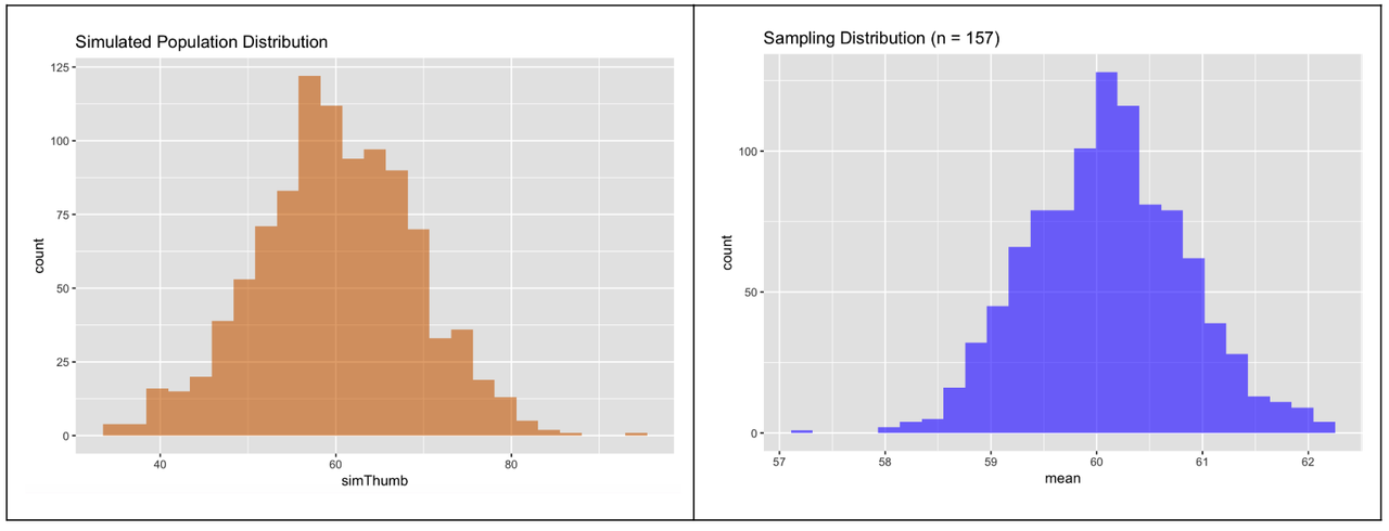
At first glance, they look fairly similar: normal shape, centered somewhere around 60. What about spread? Do these distributions have similar variation?

The sampling distribution (in blue) is actually less spread out. But it’s hard to see this from the side-by-side histograms. The reason for this is that R, which is trying to help you make a pleasing graph, adjusts the scaling of the x-axis so the histogram mostly fills up the available space.

If we want to produce histograms that are easier to compare visually, we can tell R how to scale the x-axis, and scale it the same for the two histograms. So, for both histograms, let’s chain on this additional code after the gf_histogram() function:

gf_lims(x = c(25,95))

We have added the code below to set the x-axis to go from 25 to 95 for the histogram of the simulated population (simThumb from simpop). Modify the code below that to make a histogram of the sampling distribution (mean from SDoM) scaled in the same way. Feel free to cut and paste! Cutting and pasting is an important part of coding!

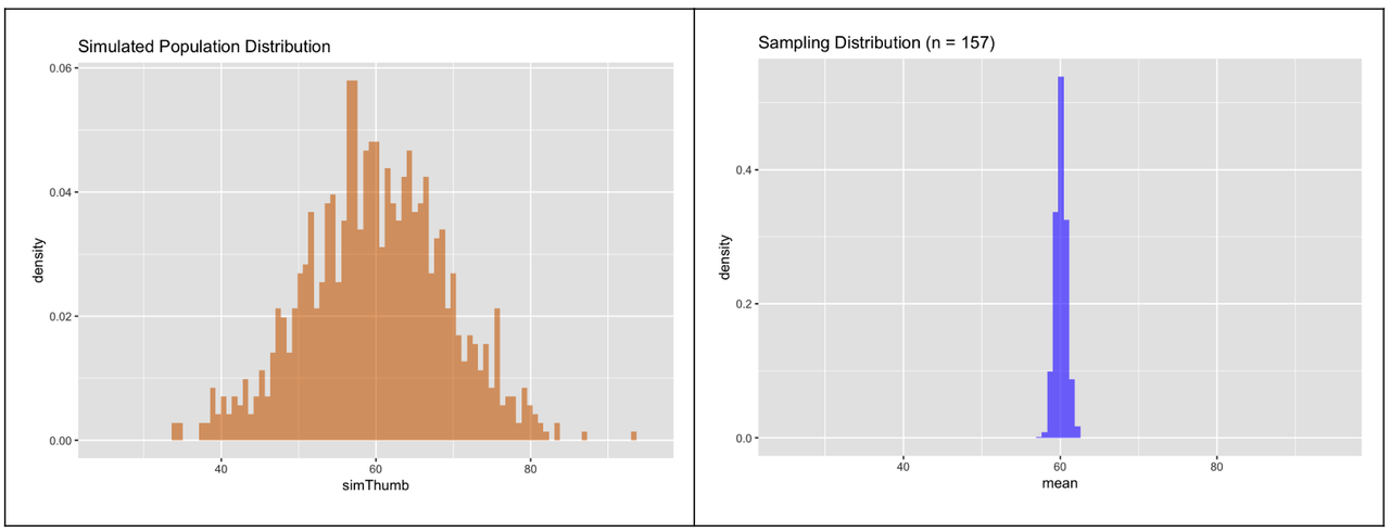
Now when we put the two histograms side-by-side on the same scale we can clearly see that the sampling distribution of means for samples of n=157 is quite a bit less spread out than the simulated population distribution.

When calculating probabilities from distributions, it is critical to pay attention to the exact question being asked. Questions about individual scores are answered in reference to the distribution they come from—the population distribution. Questions about means of samples are answered in reference to sampling distributions, because sampling distributions are the ones that generate sample means.