Course Outline
-
segmentGetting Started (Don't Skip This Part)
-
segmentStatistics and Data Science: A Modeling Approach
-
segmentPART I: EXPLORING VARIATION
-
segmentChapter 1 - Welcome to Statistics: A Modeling Approach
-
segmentChapter 2 - Understanding Data
-
segmentChapter 3 - Examining Distributions
-
segmentChapter 4 - Explaining Variation
-
segmentPART II: MODELING VARIATION
-
segmentChapter 5 - A Simple Model
-
segmentChapter 6 - Quantifying Error
-
segmentChapter 7 - Adding an Explanatory Variable to the Model
-
segmentChapter 8 - Models with a Quantitative Explanatory Variable
-
segmentPART III: EVALUATING MODELS
-
segmentChapter 9 - Distributions of Estimates
-
segmentChapter 10 - Confidence Intervals and Their Uses
-
segmentChapter 11 - Model Comparison with the F Ratio
-
11.5 Type I and II Error
-
segmentChapter 12 - What You Have Learned
-
segmentFinishing Up (Don't Skip This Part!)
-
segmentResources
list full book
11.5 Type I and II Error
We have said before that models are always wrong—they don’t perfectly represent the true state of the world, and statistical models are no exception. All we can hope for is that we can identify some models that are less wrong than others, and that some model we can fit will be better than no model at all.
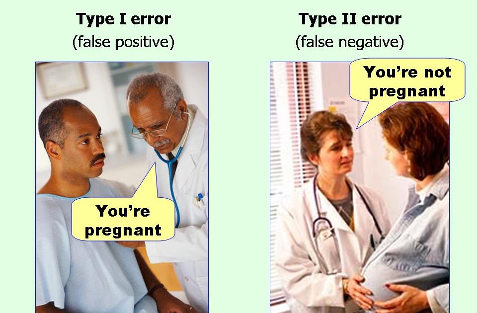
It’s also true that in the case of statistical models there are different ways of being wrong. Two of these ways of being wrong are referred to, not surprisingly, as Type I and Type II error. To understand these different ways of being wrong, let’s look at the table below.
| Model We Adopt Based on Data | What’s Really True | |
|---|---|---|
| Empty Model (\(\beta_1 = 0\)) | Complex Model (\(\beta_1 \neq 0\)) | |
| Empty Model | Yay us! | Type II Error |
| Complex Model | Type I Error | Yay us! |
There’s a big “if” behind this table: it assumes that we know what is really true, which we don’t. But let’s just imagine two alternative worlds: one where the empty model is true (the left column) and one where the complex model is true (the right column). What this thought experiment shows us is how our decision to adopt the complex model or stick with the empty model can be wrong, depending on what is really true.
The column on the left is where we have been focused with our hypothesis testing and p-value. The reason we have focused here is simply that we know how to simulate a distribution as if the empty model were true. If the empty model were true, then the F statistic we observe for our sample must have occurred just by random chance.
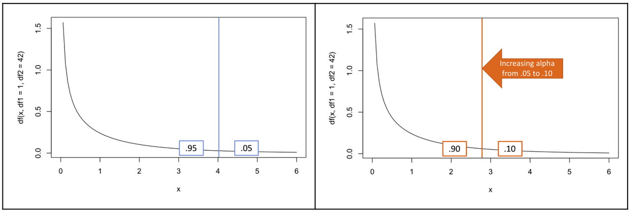
If we calculate an F statistic of 4 or greater, we rule out the empty model and adopt the complex model instead. We do this because there is a less than .05 chance that we would have obtained an F of 4+ if the empty model were correct (i.e., if \(\beta_1\) were exactly equal to 0). But while this gives us 95% confidence in our decision to adopt the complex model, there is still a .05 chance that we are wrong. Even though our chance of being wrong is low, we could be wrong. If it turns out we are wrong, we have made a Type I error.
Now let’s look at the right-hand column of the table, where the complex model is actually true (meaning that \(\beta_1\neq0\)). If this is the case, and we reject the empty model, good for us! We made the right decision. But if the complex model is true and we continue with the empty model (i.e., fail to reject it), then we have made a Type II error.
If we retain the empty model (this corresponds to the row marked “Empty model” in the table above), then the only kind of error we could be making is a Type II error. In a Type II error, the empty model is wrong, but we keep it anyway. If we adopt the complex model (thus rejecting the empty model), and we are wrong (i.e., the empty model is actually true), then we are making a Type I error.
We can calculate the exact probability of making a Type I error because we know how to simulate a distribution where randomness is the Data Generating Process. We construct a sampling distribution based on the null model, and locate our observed F within that sampling distribution. We cannot, however, directly calculate the probability of a Type II error, simply because there are many possible values that \(\beta_1\) could take if it were not equal to 0.
The most important thing to know about Types I and II error is that they are related.

The two F distributions above are the same (df1 = 1, df2 = 42). But we have shifted the boundary of what counts as unlikely from .05 to .10, and thus have increased our alpha level. Type I error is increased because we are going to end up rejecting the null model more, because lower Fs are going to be counted as “unlikely”. If we lower our standards of rejecting the empty model, then we’re going to reject the empty model more, and some of those times we will be wrong (Type I).
If we raise our standards of rejecting the empty model, then we’re going to keep the empty model more and some of those times we will be wrong (Type II). If you lower your risk of a Type I error by reducing the alpha level you are willing to accept as reason to reject the empty model, you are increasing your chance of making a Type II error.
These mistaken outcomes are linked: if you try to reduce one type of error, you raise the likelihood of the other type of error. You just can’t win either way.
