10.4 A Confession, and the t Distribution
So here is a tiny confession. We’ve been kind of (but not really) lying to you. We’ve been saying that a 95% confidence interval is roughly plus or minus two standard errors from the estimate. But as you may have guessed, it’s not exactly two standard errors.
It’s actually 1.96 standard errors. In our view, 2 is close enough to 1.96 and 2 is much easier to multiply by in your head. But when you ask R to calculate the confidence interval it will use 1.96 standard errors above and below the mean, and you will get a more precise estimate of the confidence interval.
There is one more thing, though. You might also be wondering—why don’t they just shorten the name of that confidence interval function to confint() rather than confint.default()?
That is a good question that brings us to another tiny technicality. As you saw in the previous chapter, the normal distribution isn’t always going to be the best mathematical model for a sampling distribution. When your sample size is fairly large, you can assume the sampling distribution is normal. But if the sample size is small or if the \(\sigma\) of the DGP is unknown (which it generally is), you’ll have more variation in your sampling distribution than is modeled by the normal distribution.
What do we do then? We use the t distribution, which is very similar but slightly more variable than the normal distribution (also called the z distribution). The t distribution has a slightly different shape depending on the degrees of freedom used to estimate \(\sigma\). And for very large samples, the t distribution looks exactly like the normal distribution. Bottomline: we usually use the t distribution because it can act like the normal distribution when appropriate.
The t distribution, like the standard normal distribution, is a mathematical probability function that is a good model for sampling distributions of the mean. It’s just a little more variable, that’s all.
We now know that if our sampling distribution was assumed to be normal, then the margin of error is 1.96 standard errors away from the estimate. When we express this margin of error in units of standard error (rather than in mm), we call it the critical z score.
Let’s try to think about what this distance would be if we used the t distribution instead of the z distribution. In other words, what would the critical t score be? Would it be bigger or smaller than 1.96?
A function called xqt() will take in the proportion you would like to see in one tail (e.g., .025) and the degrees of freedom (which, for now, will be n-1) and tell you the critical t score—the margin of error, in units of standard error.
For a very large sample (like 1,000 data points), this code will return something very close to 1.96 (check the R Console as well as the plot).
xqt(.025, df = 999)
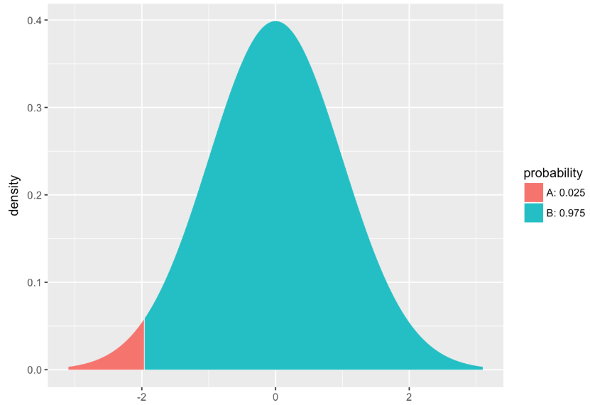
[1] -1.962341Let’s try that. Run the code below.
      packages <- c("mosaic", "Lock5withR", "Lock5Data", "supernova", "ggformula", "okcupiddata")
      lapply(packages, library, character.only = T)
      # Run this code
      xqt(.975,df=999)
      # Run this code
      xqt(.975,df=999)
      ex() %>% check_output_expr("xqt(.975, df=999)")
      success_msg("Super!")
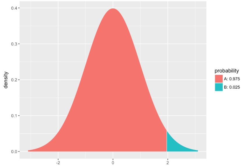
[1] 1.962341Let’s take a look at the critical t score for different sample sizes.
      packages <- c("mosaic", "Lock5withR", "Lock5Data", "supernova", "ggformula", "okcupiddata")
      lapply(packages, library, character.only = T)
      # Try finding the critical t in these different situations

      # When the sample size is 500
      xqt(.975,df=)

      # When the sample size is 157 (like in our Fingers data)
      xqt(.975,df=)

      # When the sample size is 50
      xqt(.975,df=)

      # When the sample size is 20
      xqt(.975,df=)
      xqt(.975,df=499)
      xqt(.975,df=156)
      xqt(.975,df=49)
      xqt(.975,df=19)
      ex() %>% {
        check_function(., "xqt", index = 1) %>% check_result() %>% check_equal()
        check_function(., "xqt", index = 2) %>% check_result() %>% check_equal()
        check_function(., "xqt", index = 3) %>% check_result() %>% check_equal()
        check_function(., "xqt", index = 4) %>% check_result() %>% check_equal()
        }
      success_msg("Keep up the great work!")
| Degrees of Freedom (df) |
Critical t (the critical distance in units of standard error) |
|---|---|
| 499 | 1.964729 |
| 156 | 1.975288 |
| 49 | 2.009575 |
| 19 | 2.093024 |
The function confint() uses the t distribution to estimate the margin of error. So it will adjust for the size of your sample automatically. The function we tried out before, confint.default() uses the z distribution (which does not change with degrees of freedom).
Try out both of these functions in the code window below. Is the confidence interval based on the t distribution (confint()) slightly bigger than the one based on the normal distribution?
      packages <- c("mosaic", "Lock5withR", "Lock5Data", "supernova", "ggformula", "okcupiddata")
      lapply(packages, library, character.only = T)
      Thumb.stats <- favstats(~ Thumb, data = Fingers)
      SE <- Thumb.stats$sd/sqrt(Thumb.stats$n)
      Empty.model <- lm(Thumb ~ NULL, data = Fingers)
      # This will calculate CI based on the normal distribution.
      confint.default(Empty.model)

      # Write code to calculate CI based on the t distribution.
      # Write code to calculate CI based on the t distribution.
      confint(Empty.model)
ex() %>% check_function("confint") %>% check_result() %>% check_equal()
               2.5 %   97.5 %
(Intercept) 58.73861 61.46871
2.5 % 97.5 %
(Intercept) 58.72794 61.47938Indeed, using the t distribution to approximate sampling distributions leads to a slightly wider confidence interval (the lower bound is a little smaller, the upper bound is a little bigger). But at the end of the day, for samples that are fairly large, none of these technical details make a huge difference. That’s why, even after going through all these details, we still think of the 95% confidence interval as being about plus or minus two standard errors from our estimate.
Bottom line, all you need to use is confint(). It will give you the best estimate of the confidence interval regardless of sample size.
One last thing: sometimes you may just want the lower bound of a confidence interval, or the upper bound. If we tell you that the function confint() returns a vector of two numbers (the first being the lower bound and the second, the upper bound) you could probably figure out how to just get one or the other. Run the following code to see what we mean.
      packages <- c("mosaic", "Lock5withR", "Lock5Data", "supernova", "ggformula", "okcupiddata")
      lapply(packages, library, character.only = T)
      Thumb.stats <- favstats(~ Thumb, data = Fingers)
      SE <- Thumb.stats$sd/sqrt(Thumb.stats$n)
      Empty.model <- lm(Thumb ~ NULL, data = Fingers)
      # Try running this code
      confint(Empty.model)[1]
      confint(Empty.model)[2]
      # Try running this code
      confint(Empty.model)[1]
      confint(Empty.model)[2]
      ex() %>% {
        check_function(., "confint", index = 1) %>% check_result() %>% check_equal()
        check_function(., "confint", index = 2) %>% check_result() %>% check_equal()
        check_output_expr(., "confint(Empty.model)[1]")
        check_output_expr(., "confint(Empty.model)[2]")
      }
      success_msg("Awesome!")
[1] 58.72794[1] 61.47938The code confint(Empty.model)[1] will return the lower bound and confint(Empty.model)[2] will return the upper bound.