9.3 Simulations from a Different DGP, and Learning to Say “If…”

In our die rolling simulations, we didn’t start with a sampling distribution. We started, first, by thinking about the DGP, then the population distribution that we thought would result from the DGP. After that we simulated, using the resample() command, the distributions of some individual samples generated by the DGP. And finally, we simulated the sampling distribution of means for samples of a particular size (n=24).

We have learned, through these simulations, a lot about rolling die! But more importantly, we learned that each of these distributions (population, sample, and sampling) can have very different characteristics from each other. Sample distributions will often look quite different from the population distribution. We could see this clearly in the case of dice, because we know what the population distribution looks like. If we only had one sample, and an unknown population distribution, we would need to be cautious in interpreting our sample distribution.

We also saw that sampling distributions are really quite divorced from sample distributions. The unit that makes up a sampling distribution (in our example, the means of different samples) doesn’t even appear in a distribution of data. It is something we calculate, once per sample, after the fact. To get a sampling distribution we have to imagine selecting a large number of samples from a population distribution that generally is not known.

All of this gets very hypothetical, as there are many unknowns. Our sample distribution is known, but that’s about it. From there we must make assumptions, saying “If…” This is the world of simulation. Once we have some ideas, or hypotheses, about the DGP, we can then use computers to simulate the construction of a sampling distribution. This allows us to say, “If the DGP is like this, then here is what the distribution of sample statistics could look like.”

From there we can go back to our data, our particular sample, and see where it would fit if the assumptions we made are true. And, we don’t have to stop there. We can change our assumptions and start the simulations again. As we will see, this is an incredibly powerful way of thinking.

In this section we are going to explore simulations from a different DGP, one we will assume can be modeled by a normal distribution. Die rolls are nice because we know a lot about the DGP that controls them. But most things we study are not generated by a uniform DGP. Most things are more like thumb length: caused by many factors, measured and unmeasured, and normally distributed. Let’s see how much we can understand about thumb length through simulations.

Thumb Length: Simulating a Random Sample from a Population

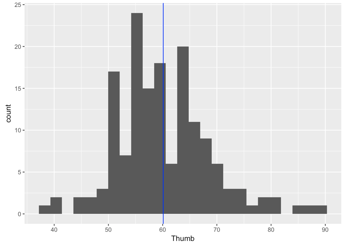
Recall we collected a sample of n=157 thumb lengths of undergraduate students. Just to review, let’s look at a histogram of our sample distribution. This is real, not simulated.

Now let’s start thinking about some hypotheses to guide our simulations. Let’s assume, just for argument’s sake (remember, we are starting with “If…”) that the distribution of thumb length in the population is normally shaped. It’s true that our sample distribution is not perfectly normal. But by now you have seen many examples of weirdly shaped sample distributions coming from normal population distributions. And besides, normal seems to make sense in this case.

Here are the favstats for Thumb from our sample.

min Q1 median Q3 max     mean       sd   n missing
 39 55     60 65  90 60.10366 8.726695 157       0

Let’s just use these sample statistics to estimate our population parameters. We will assume that the mean of the population is 60.1, and the standard deviation, 8.73. We know that these estimates are unlikely to be true. But we also know that they are the best unbiased estimates we can come up with based on our single sample. So we will use them.

Even if we assume this simple DGP, if we simulate drawing multiple samples, the individual samples generally will not look like our hypothesized population distribution. Let’s try some simulations and see what happens.

Normal distributions are very easy to simulate because they are mathematically defined by just two parameters.

Since we are going to need the mean and standard deviation of our sample, let’s start by saving the favstats() for Thumb from the Fingers data frame in an R object called Thumb.stats. We’ll use these to define our hypothesized normal population distribution, and by saving them we won’t need to keep typing them in.

min Q1 median Q3 max     mean       sd   n missing
 39 55     60 65  90 60.10366 8.726695 157       0

In order to simulate picking a random sample from a normal distribution, we use the function rnorm(). The r in front of this function stands for “random sample” and the norm stands for “normal distribution.” We need to tell rnorm() how large a sample to generate, and from which normal distribution to generate it (defined by its mean and standard deviation).

We will start by generating a sample of one data point:

rnorm(1, mean = Thumb.stats$mean, sd = Thumb.stats$sd)

Go ahead and generate one data point by running this code.

[1] 54.63679

Using the same assumptions about the DGP, let’s simulate drawing some more data points.

Modify the code below to simulate randomly drawing 20 thumb lengths from the hypothesized population.

 [1] 54.63679 61.70626 52.81139 74.02519 62.97918 52.94369 64.35731
 [8] 66.54680 65.12833 57.43863 73.29651 63.50571 54.68229 40.77665
[15] 69.92059 59.71154 59.96237 68.34023 67.27021 65.28646

These 20 data points do not constitute a sampling distribution but, instead, just a single sample of 20 thumb lengths randomly selected from the assumed DGP. If it were a sampling distribution of means, each number would represent the mean of a sample. But so far, we have not even calculated a mean of this sample. So this is just a sample distribution, that is, a single sample of n=20.

It would be easier to look at these simulated thumb lengths if they were in a histogram. Let’s generate a lot of thumb lengths (let’s do 1,000) using our hypothesized DGP and save them into a variable simThumb. Then put simThumb into a data frame called simpop (short for simulated population). Finally, write code to make a histogram of this simulated population.

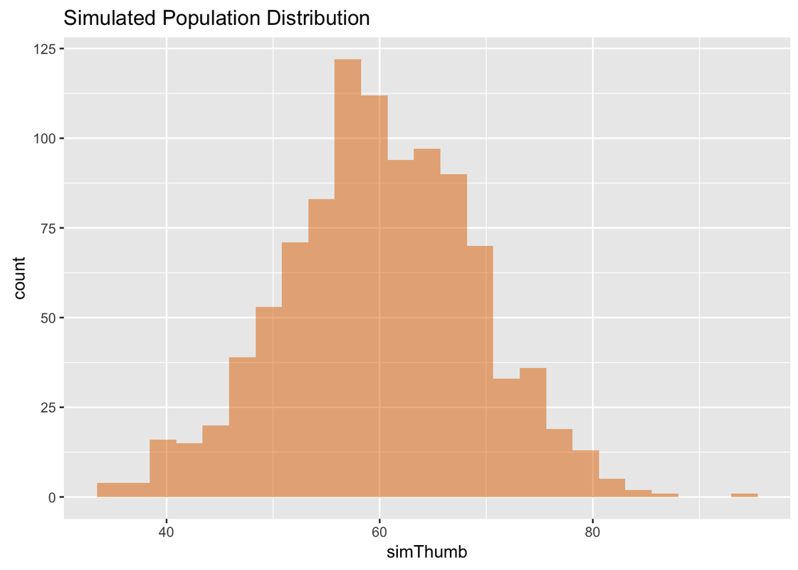
Note that the simulated distribution looks very close to normal in shape—just like the population shape we hypothesized. You can also see that even a DGP centered around 60.1 mm, with a standard deviation of 8.73, could still generate thumb lengths as large as 80 mm or as small as 40.

A simulation this large starts to give us a sense of what the population might look like if it were generated by our hypothesized DGP. We can say: “If the DGP is consistent with our estimates and assumptions, here is what the population distribution of thumbs might look like.”

We have generated these 1,000 thumb lengths by randomly picking numbers from a normal distribution defined to have the same mean and standard deviation as our Thumb data from Fingers (mean = 60.1, standard deviation = 8.73).

Go ahead and calculate the favstats() for simThumb in the simpop data frame in R.

     min       Q1   median      Q3      max     mean       sd     n missing
33.85334  54.0179 59.7954 66.11136 93.35478 60.00201 9.031394  1000       0

The simulated population has a mean of about 60, which is close to the mean we set for the simulated normal DGP (60.1). The standard deviation of this distribution is also quite close to the one that we set. This makes sense because we told rnorm() the mean and standard deviation it should assume for the simulated normal DGP. (NOTE: Because this is a random simulation, the exact numbers you get will be slightly different each time you run the code.)

Using “If…” thinking, we have been able to simulate a distribution that helps us think about what the population would look like if the DGP were a particular normal distribution. But simulating a population of individuals does not directly help us understand sampling variation. For that, we need to use the same “If…” simulation strategy, but generate multiple samples instead of a single, albeit large, sample of individual thumb lengths.