10.3 Using the Normal Distribution to Construct a Confidence Interval

We have introduced two methods of creating sampling distributions: simulation and bootstrapping. We now will introduce one more method: modeling the sampling distribution with a mathematical probability distribution, the normal curve.

We used the normal curve back in Chapter 6 as a way to calculate probabilities in the population distribution. Not all population distributions are normal, but when they are, the normal curve gives us an easy way to calculate a probability. If we model the distribution of Thumb length with the normal curve, we can simply use the xpnorm() function to tell us the probability of the next randomly selected individual having a Thumb length greater than 65 mm, for example.

Because of the Central Limit Theorem, the normal curve turns out to be an excellent model for a sampling distribution of means. Even if the population distribution is not normal, the sampling distribution is well modeled by the normal curve, especially when sample sizes are larger. And before we had easy access to computers, everyone used the normal model, and the Central Limit Theorem, as a way to estimate the standard error.

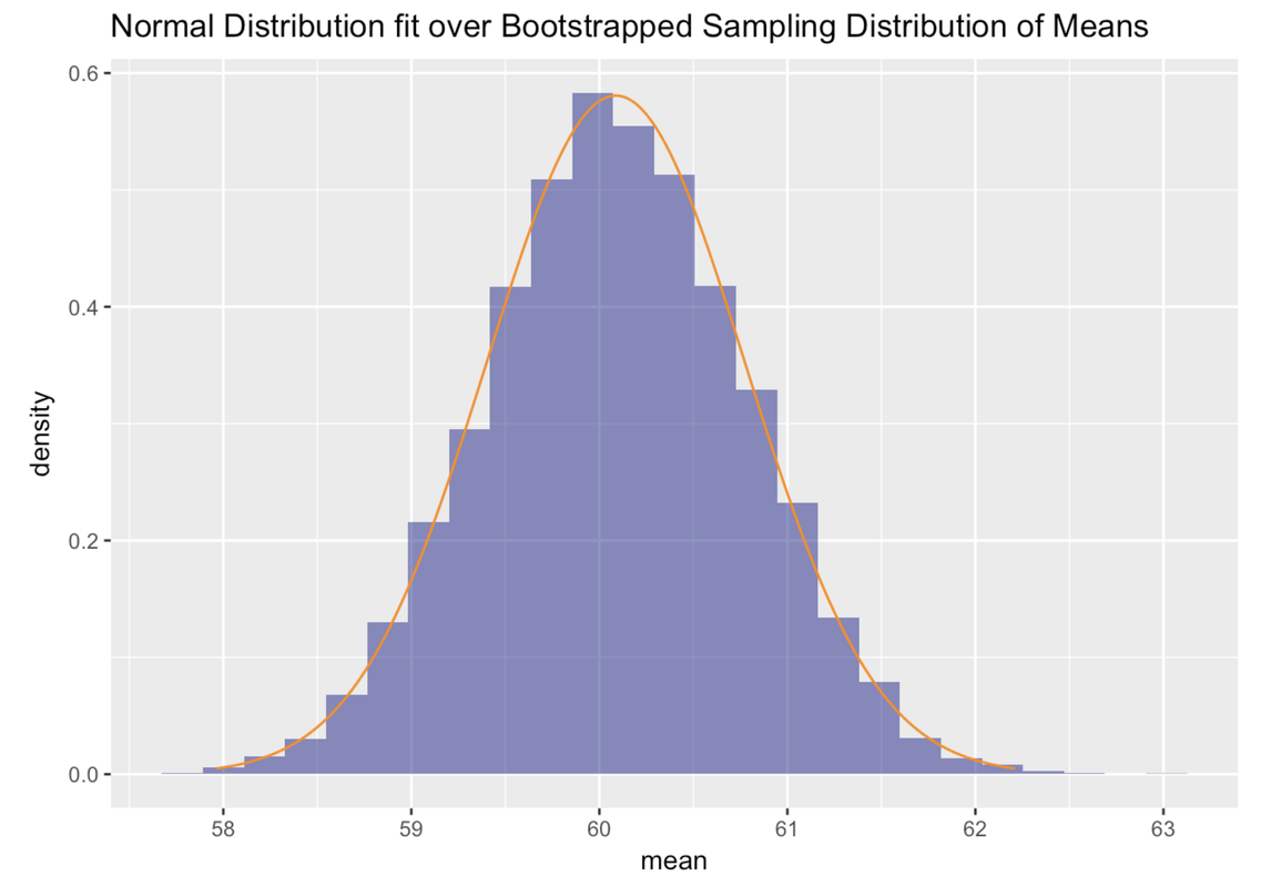
Here we will use some R code to fit the normal curve over the bootstrapped sampling distribution of means. As you can see, the normal curve fits pretty well.

gf_dhistogram( ~ mean, data = bootSDoM, fill = "darkblue") %>%
gf_dist("norm", color="darkorange", params=list(mean(bootSDoM$mean), sd(bootSDoM$mean)))

Using the Normal Model

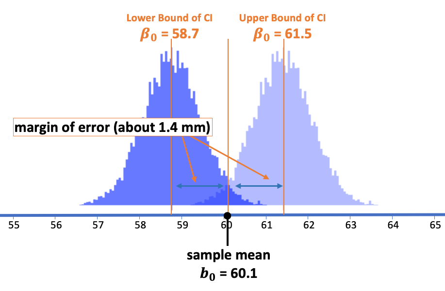
The logic of using the normal model is exactly the same as using a simulated or bootstrapped sampling distribution. What we are trying to find out is the range of possible population means (represented in the sampling distributions below) that could have produced the particular sample mean we observed in our study.

In reality, there is no population mean for which our sample mean is impossible. To say that another way, our sample mean is possible under any population mean. Instead of focusing on what is possible, we focus on what is most probable. If our sample mean is within the range of the most (95%) probable sample means for a specific population mean, that population mean is included in the 95% confidence interval.

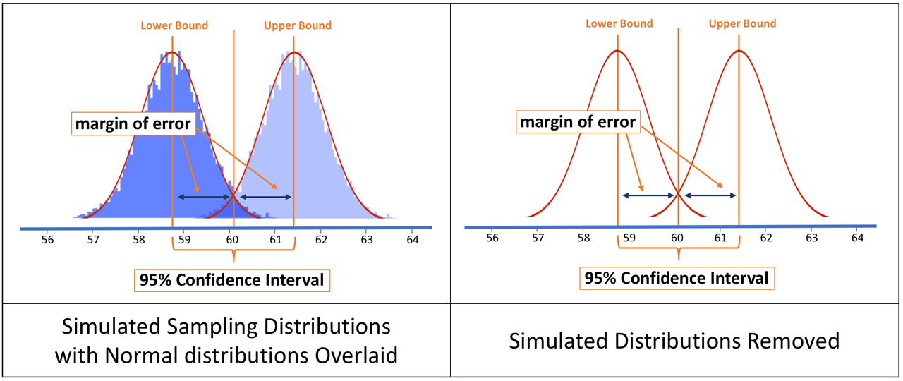
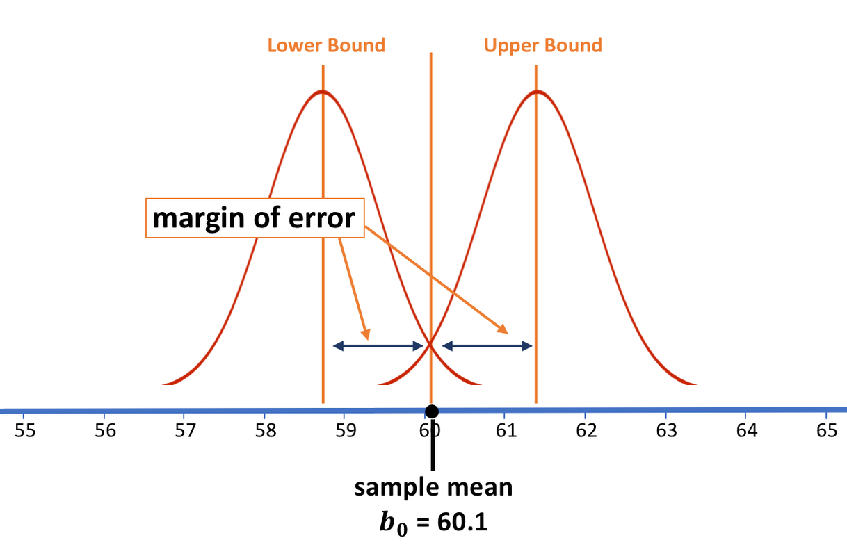
The margin of error represents how far off the true population mean could be from our estimate. We use sampling distributions to find the margin of error, the distance between the hypothesized lower bound of possible population means and the 2.5% cutoff point above which it would be unlikely for our sample to have been drawn. The same margin of error lies between the hypothesized upper bound and its 2.5% cutoff point.

If we wanted to find out the confidence interval (the actual values of the lower and upper bound), subtracting the margin of error from the sample mean will tell us exactly where the lower bound of the confidence interval is. We could follow a similar method to find the upper bound.

Using Standard Errors as the Unit

With simulated and bootstrapped sampling distributions, we constructed sampling distributions, literally arranged the means in order, and then looked at the cutoffs (the 25th and 975th means) to find the confidence interval. We used the confidence interval to figure out the margin of error.

With the normal distribution we must take a different approach. The normal distribution is a mathematical model, so there is nothing to order or count. We need a different way to calculate the margin of error and the two 2.5% cutoff points.

A rough way to do this is to use the “empirical rule,” which we first introduced in Chapter 6. We’ve reproduced the figure from Chapter 6 below.

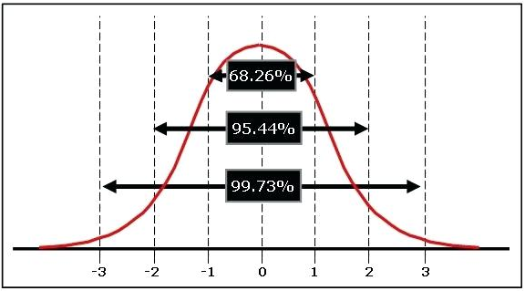
According to the empirical rule, 95% of the area under the normal curve is within two standard deviations, plus or minus, of the mean of the distribution. So, even before we know the standard deviation of our sampling distribution (which we call the standard error), we know that the lower cutoff point is going to be approximately two standard errors below the sample mean, and the upper cutoff will be two standard errors above the sample mean.

Directly Calculating the Standard Error using the Central Limit Theorem

We know how wide the confidence interval will be in standard errors (2 on each side of the sample mean; a total of 4). But if we want to know the width of the confidence interval in millimeters, we will need to figure out how big the standard error of the sampling distribution is.

The Central Limit Theorem provides a formula for calculating the standard error of a sampling distribution. Do you remember what the formula is for calculating standard error?

Because we don’t know what the true value of \(\sigma\) is, we can estimate the standard error by dividing the estimated standard deviation based on our sample (\(s\)) by the square root of n (the sample size, which in this case is 157).

Use the code window below as a calculator to estimate the standard error of Fingers$Thumb. Note, we have written code to save the favstats of thumb lengths in Thumb.stats.

[1] 0.696466

Hey, that’s very close to what we thought the standard error would be (.7, half of the margin of error we got from simulations – 1.4)!

So now let’s go back to our original question: Given the sample mean we observed (our estimate), what is the range of possible values within which we could be 95% confident that the true population mean would lie?

Now, using the standard error you just calculated, figure out the approximate 95% confidence interval around the observed sample mean. Is it close to the confidence interval we got from simulation and bootstrapping (58.7 to 61.5)?

[1] 61.49659

[1] 58.71073

The confidence interval (58.7, 61.5) is very similar to what we got from simulations and bootstrapping!

Using R to Calculate the Confidence Interval

Although we have been focusing on the confidence interval for the mean, it is important to note that the mean is just one parameter we can estimate. Ultimately, we can create confidence intervals for all kinds of parameters, not just the mean.

As you may recall, the simplest model (what we have been calling the empty model), only estimates one parameter, the mean. Remember, we used the lm() function to fit this one parameter model to our Fingers data and then save it as Empty.model.

Empty.model <- lm(Thumb ~ NULL, data = Fingers)

We can print out the parameter estimates by just typing the name of our saved model.

Empty.model

Call:
lm(formula = Thumb ~ NULL, data = Fingers)

Coefficients:
(Intercept)
       60.1

The function confint.default() takes a model as its input, and then computes the 95% confidence intervals for the parameters of that model using the normal distribution. Try running the code below.

               2.5 %   97.5 %
(Intercept) 58.73861 61.46871

Ta da! You might be thinking: Why didn’t they just lead with this? Why did we have to go through simulations and bootstrapping? We could have just told you about this function from the beginning. But then you wouldn’t have had the rich understanding of what these numbers meant, or what this function is doing.