9.6 Reasoning With Sampling Distributions

Now that you have an idea of what sampling distributions are, let’s find out how we can use them to reason about data. There are two moves we can make in this regard: the first, which we will call reasoning forward, is easier to understand. The second, reasoning backwards, is harder to understand, but much, much more useful. Fortunately, understanding the first move will help you understand the second one.

Both reasoning forward and reasoning backward rely critically on the use of “IF…”. Using the word IF is the most important part of using sampling distributions to evaluate estimates and models.

Reasoning Forward

For example, we can ask, if the mean thumb length of the population is 60.1 mm, how likely is it that we would randomly draw a sample of n=157 with a mean higher than 61 mm? (Where did we get 61 mm? We were just curious about it, that’s all. You could wonder about any mean.)

To answer this question, we need a sampling distribution. Why? Because our question is about the likelihood of getting a mean greater than 61 mm, and so the likelihood needs to be assessed in reference to the sampling distribution of means.

We can simulate a sampling distribution, as we did before, assuming a normal distribution with \(\mu=60.1\) and \(\sigma=8.73\). We’ll use this R code to generate a sampling distribution of 1,000 means of randomly selected samples of n=157, and then plot the sampling distribution in a histogram:

SDoM <- do(1000) * mean(rnorm(157, mean = Thumb.stats$mean, sd = Thumb.stats$sd))
gf_histogram(~ mean, data=SDoM, fill = "blue")

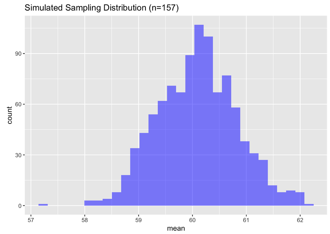
Look at the sampling distribution, and now go back to the question we were trying to answer: If the population has a mean of 60.1 and a standard deviation of 8.73, what is the likelihood of getting a random sample of n=157 with a mean greater than 61?

It’s easier to visualize the answer to this question if you shade with a different color all of the simulated samples with means greater than 61. R provides an easy way to do this just by adding another argument (fill = ~mean >= 61) to the gf_histogram() function, like this:

gf_histogram(~ mean, data=SDoM, fill = ~mean >= 61)

This addition says: check each mean to see if it is greater than or equal to 61. If it is, fill with one color; if it isn’t, fill with another color.

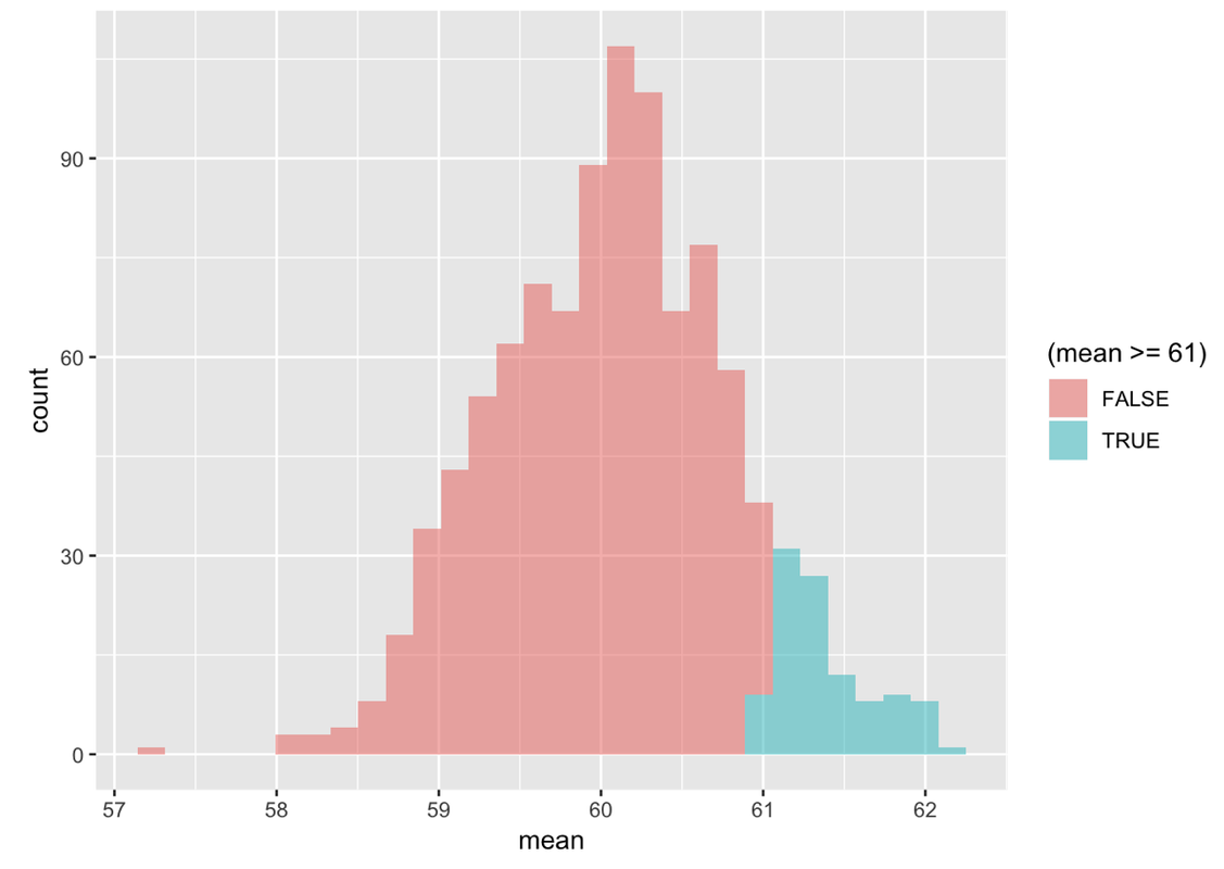
Like the previous one, this histogram represents 1,000 simulated samples of n=157 from a population with mean of 60.1 and standard deviation of 8.73. But now all of the simulated samples with means of greater than or equal to 61 have been shaded green. So, if you can eyeball the proportion of the histogram that is shaded green, you can get a sense of how likely it would be to draw a sample of 157 thumbs with an average length greater than or equal to 61 mm.

To get the exact number of means of the 1,000 in our simulated sampling distribution that are greater than or equal to 61, we can use the tally() function.

tally(~ mean >= 61, data = SDoM)

mean >= 61
 TRUE FALSE
  105   895

Since we conveniently simulated 1,000 samples, we can see that .105 (or about .10) of means are larger than or equal to 61. But we can also modify tally to format the output as proportion rather than frequency. Modify the following code to return proportions.

mean >= 61
 TRUE FALSE
0.105 0.895

Using the same sampling distribution (SDoM), see if you can answer a new question: If the population distribution is normal with a mean of 60.1 and standard deviation of 8.73, what are the chances of randomly selecting a sample of n=157 with a mean of greater than or equal to 65 mm?

First, modify the code below to answer this question visually using a shaded histogram.

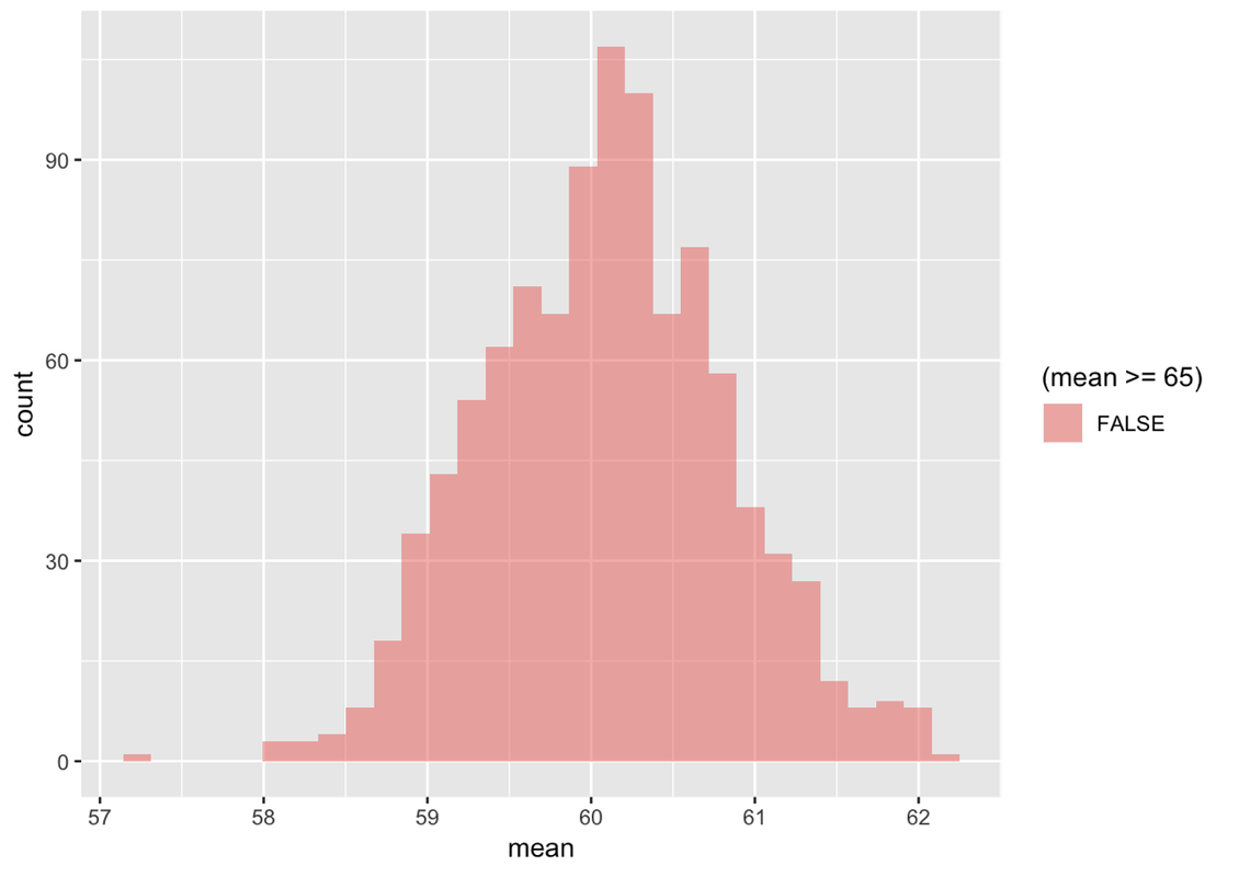
In statistics, we rarely say that there is a 0% chance of something because we are trying not to be wrong. After all, even though it’s very unlikely to roll a die 24 times and get 6 every single time, it is still possible. In situations like this, we will typically say this value (65) has a very low probability, rather than to conclude that we could never get 65 as a sample mean.

Now write a tally() command in the window below to find out exactly what proportion of the samples in your simulated sampling distribution (SDoM) had means greater than 65.

mean >= 65
 TRUE FALSE
    0     1

Just like we recommend you visually explore your data before you model it, it’s also a good idea to create a shaded histogram when reasoning forward from a sampling distribution. Even experienced statisticians make mistakes. Looking at the histogram gives us a way to check whether the output we get from R (e.g., the tally() function) is reasonable.

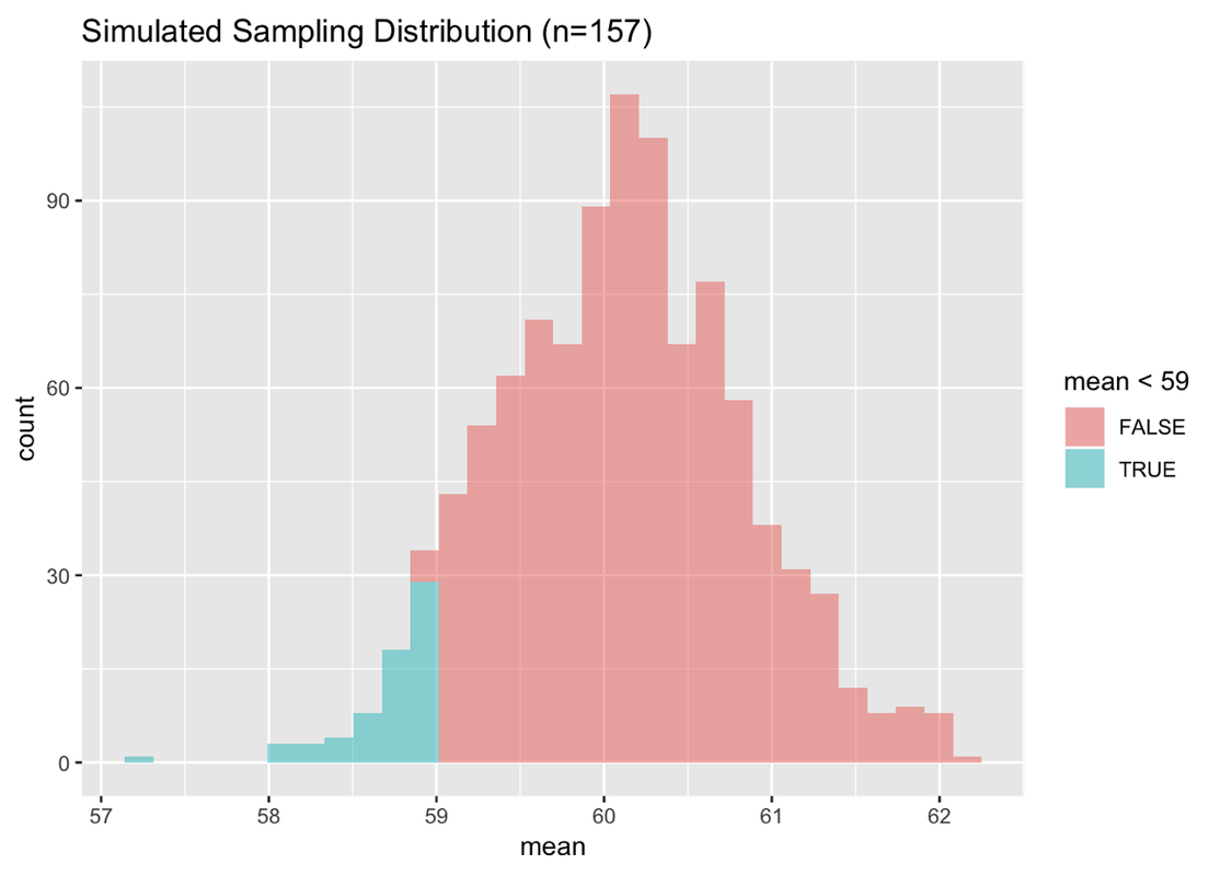
Try asking one more question of SDoM. What is the likelihood of randomly selecting a sample of n=157 from the same DGP with a mean that is smaller than 59 mm?

Use the code window below to calculate the exact proportion of 1,000 simulated samples with means smaller than 59 mm, and then also create a shaded histogram to confirm your result.

mean < 59
 TRUE FALSE
0.066 0.934

In reasoning forward, we:

• Hypothesize a DGP and/or population distribution

• Generate a sampling distribution from the assumed DGP/population

• Use the sampling distribution to calculate the likelihood of getting certain sample means if the assumptions about the DGP/population are true.

In reasoning forward, the distribution triad is ordered like this: (1) DGP/population, (2) sampling distribution, (3) sample. You can think of a hypothetical DGP/population in a number of ways. The hypothetical DGP can be based on what you know about the process (like in die rolls); you can base it on a number you are interested in; or you can use information from your sample to help you estimate what the population might be. The important point is that you start by assuming something about the population first. We end by comparing our sample against the possible samples.