10.8 Using Confidence Intervals to Evaluate a Regression Model

As you can see by now, we can construct a sampling distribution, and thus a confidence interval, for any parameter we can estimate from data. We started with our estimate of the mean (\(b_{0}\)), and then moved on to our estimate of the difference in means between two groups (\(b_{1}\)).

In our two-group example, we introduced an approach to using confidence intervals to evaluate models. We started by specifying a complex model (for example, a model with one more parameter than the empty model). We then fit the complex model (i.e., calculated the best parameter estimates).

Because the particular estimates we calculated were just one possible set of estimates that we could have gotten, depending on sampling variation, we constructed a confidence interval around our estimates. The confidence interval shows us the possible range of worlds (\(\beta\)s) where our sample estimate would be considered likely. We constructed a sampling distribution around the additional parameter, the one that differentiated the complex model from the empty model (in this case, \(\beta_1\), or the increment from Short to Tall).

Finally, we checked to see if the confidence interval around the additional parameter estimate included 0. If it did include 0, we would just stick with the empty model. It is, after all, simpler! Even though your estimate might be greater than 0, it could have resulted from random variation in sampling. Thus, there is no strong evidence from our data that would cause us to rule out the simpler model in favor of the more complex model.

If it did not include 0, however, which in our case it did not, then we could reject the empty model and adopt the more complex one. To use the language of statistical significance testing, we would say that the complex model was significantly better than the empty model. Or, similarly, we could say that the parameter representing the group difference was significantly different from 0.

Application to the Regression Model

Let’s see if we now can apply this same approach to evaluating a regression model. We used regression, you may recall, to model the relationship between a quantitative explanatory variable and a quantitative outcome. We would use a regression model, for example, to represent the relationship between height in inches (the explanatory variable) and thumb length in millimeters.

What we really want to know is this: in the population, if we know someone’s height in inches, does it help us make a better prediction about their thumb length? Or would we do just as well to go with the same guess (the Grand Mean) for everyone?

We can specify the Height model like this:

\[Y_{i}=b_{0}+b_{1}X_{i}+e_{i}\]

Our model specification looks the same as the two-group model, but by now you know that the interpretation of the different model components will be different.

In this model, the two parameters define a best-fitting line. \(b_{0}\) represents the y intercept, or the value of Y when X equals 0. \(b_{1}\) represents the slope of the line, or the incremental value added to Y for each unit increase in X. In this case, the slope would represent the increase in thumb length in millimeters for each one-inch increase in height.

Go ahead and fit the Height model in R using lm().

From our best-fitting estimates we see that Height helps to predict Thumb in our sample. But what we really want to know is whether Height could help us predict Thumb length in the population. If \(\beta_{1}\) is actually 0, then we would not need to include Height in the model since it would be multiplied by 0 anyway. But if \(\beta_{1}\) is not equal to 0, we can reject the empty model and adopt the more complex regression model.

Since we can’t directly calculate \(\beta_{1}\), we will use \(b_{1}\) as an estimate. But estimates from samples have a problem. They vary from sample to sample. This is why we turn to sampling distributions to give us a sense of how much these estimates vary. Even though our estimate of the increment from the sample is .96 (adding on .96 mm to Thumb length for every inch of Height), in the population \(\beta_{1}\) could be less, or it could be more. How much could it vary? Could it be 0? These are the questions we can answer with the confidence interval.

The simple model to which we would compare the more complex, regression model would be this one:

\[Y_{i}=b_{0}+e_{i}\]

Using this model, we would predict each person’s thumb length to be the mean of all thumb lengths in the sample regardless of their height. If we adopted the regression model, we would be saying that the prediction is significantly better if, in addition to the mean, you use the person’s height to predict thumb length.

The difference between these two models is the slope, or \(b_{1}\). If \(b_{1}\) were equal to 0, then the complex model would be reduced to the empty model. The slope, then, is the key parameter we are interested in.

Constructing a Sampling Distribution Around the Slope

We’ve already constructed a sampling distribution around \(b_{1}\) before, for the two-group model (i.e., Height2Group). Using the same approach as before, let’s use resampling to construct a sampling distribution for the slope of the regression line. Starting with our sample, we will:

• Resample with replacement to generate a new, bootstrapped sample;

• Fit the regression model to find the slope of the best-fitting regression line (i.e., calculate a value for \(b_{1}\));

• Repeat 1,000 times;

• Record the resampled estimates in a new data frame.

Try putting all that together in the code window below. Save your 1,000 resampled slopes as bootSDob1. Print the first six lines of bootSDob1.

         b1
1 0.9610974
2 0.8647881
3 1.1550938
4 0.8639170
5 1.1547266
6 0.8751995

Use the code window to create a histogram and run favstats on b1 from bootSDob1 (you can assume bootSDob1 has already been created).

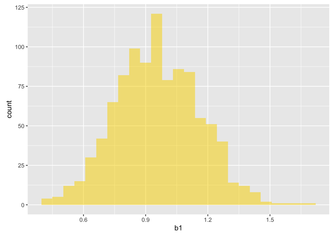
       min        Q1    median       Q3     max      mean        sd     n missing
 0.2715344 0.8287651 0.9568719 1.091199 1.68477 0.9610564 0.1965496  1000       0

Note that this sampling distribution’s center is close to our estimate of \(b_1\), .96. This is because these samples are resampled from a population that is based on our sample.

Now that we have a sampling distribution, we can construct the 95% confidence interval using one of the methods we have developed.

The first approach is simply to find the cutoff points for the confidence interval directly from the bootstrapped sampling distribution. In this code exercise, arrange b1 in bootSDob1 in order, and examine the 25th and 975th values.

[1] 1.358762

[1] 0.5816517

These cutoff points define the 95% confidence interval for the slope of the regression line. The lower bound for the slope is around .6, the upper bound is a little bigger than 1.3.

Using a Mathematical Probability Distribution to Construct the Confidence Interval for Slope

Instead of using bootstrapping to get the confidence interval around our estimate, we could just use the function confint(). This method will: 1) assume that the sampling distribution of the slope is shaped like a t distribution, 2) use the t distribution to figure out how far away the “unlikely” zone is in units of standard error (this distance will, once again, be about 2 standard errors), and 3) then estimate standard error to figure out how far away the “unlikely” zone is in millimeters.

In the code window below, fit the complex model using Height to explain variation in Thumb length. Then run confint() to find the confidence intervals around the estimates.

                  2.5 %    97.5 %
(Intercept) -27.0506830 20.391710
Height        0.6026976  1.321069

Notice that the confidence interval for slope produced by confint() using the t distribution (.60 to 1.32) is very close to the one we constructed based on our bootstrapped samples (.58 to 1.36).

Interpreting the Confidence Interval for Slope

Based on our sample, we initially estimated the slope of the regression line to be .96, meaning that the increment in thumb length for every inch in height is .96 mm.

We are interested in whether or not the true value of \(\beta_{1}\) could be 0, because it will help us compare, and choose between, two models for thumb length.

The complex model represents thumb length as a regression line. It is a two-parameter model: one for the y intercept and the other for slope. We represent the model like this:

\[Y_{i}=\beta_{0}+\beta_{1}X_{i}+\epsilon_{i}\]

If the confidence interval for slope included 0, we could decide to use the simpler, empty model. If the slope were actually 0, then \(\beta_{1}\) would be equal to 0. If that were true, then the \(\beta_{1}X_{i}\) term would become 0 and drop out, leaving us with the simple model:

\[Y_i=\beta_0+\epsilon_i\]

Note, however, that just because the confidence interval includes zero, it doesn’t mean that it is zero. The confidence interval would include a lot of numbers around zero as well.

In the case of height and thumb length, confidence interval around the slope, .6 to 1.32, does not include 0. This means we are pretty confident that the true slope in the population is not 0. Because the confidence interval around the slope did not include 0, we can, with 95% confidence, reject the simple model and adopt the complex one.

Even with the best statistical tools, we still are left with only a fuzzy idea of what the true population parameters are. Our estimates of \(\beta_{0}\) and \(\beta_{1}\) are called “best-fitting estimates” because if we had to make our best guess about these population parameters, these (\(b_{0}\) and \(b_{1}\)) are the numbers we would use.

But it is highly unlikely that these estimates are accurate indicators of the true population parameters. Confidence intervals help us to keep that in mind. By coming up with a range of possible parameters given our data, we simultaneously make use of our data, while acknowledging that our data are filled with noise—random and otherwise.

Although it might be comforting to just get one estimate instead of the range offered by a confidence interval, just using one estimate increases our likelihood of being wrong. By calculating a confidence interval, we are acknowledging the uncertainty in our estimate, and drawing boundaries around that uncertainty. Even if the interval is large, we can at least be 95% confident that the true parameter lies somewhere in that interval.

End of Chapter Survey