10.1 Finding the 95% Confidence Interval with Simulation

Now all we need to do to construct the 95% confidence interval around our estimate of mean thumb length is find the margin of error. We can do this in several ways; let’s start by using simulation.

Simulating a Sampling Distribution Centered at the Sample Mean

We just established in the previous section that the sampling distribution of means centered around our sample mean can be used to calculate the margin of error. Let’s start by simulating the sampling distribution, and then use that sampling distribution to find the margin of error.

Starting with the mean and standard deviation estimated from our sample, and the assumption that the population is normally distributed, we can simulate a sampling distribution of means for samples of n=157, centered at the estimated population mean (see picture). We’ll call the resulting data frame simSDoM to stand for “simulated Sampling Distribution of Means”.

simSDoM <- do(1000) * mean(rnorm(157, mean = Thumb.stats$mean, sd = Thumb.stats$sd))

This R code produces a data frame with 1,000 simulated sample means. The mean of this sampling distribution will be very close to 60.1, which is our estimate of \(\mu\) based on our sample.

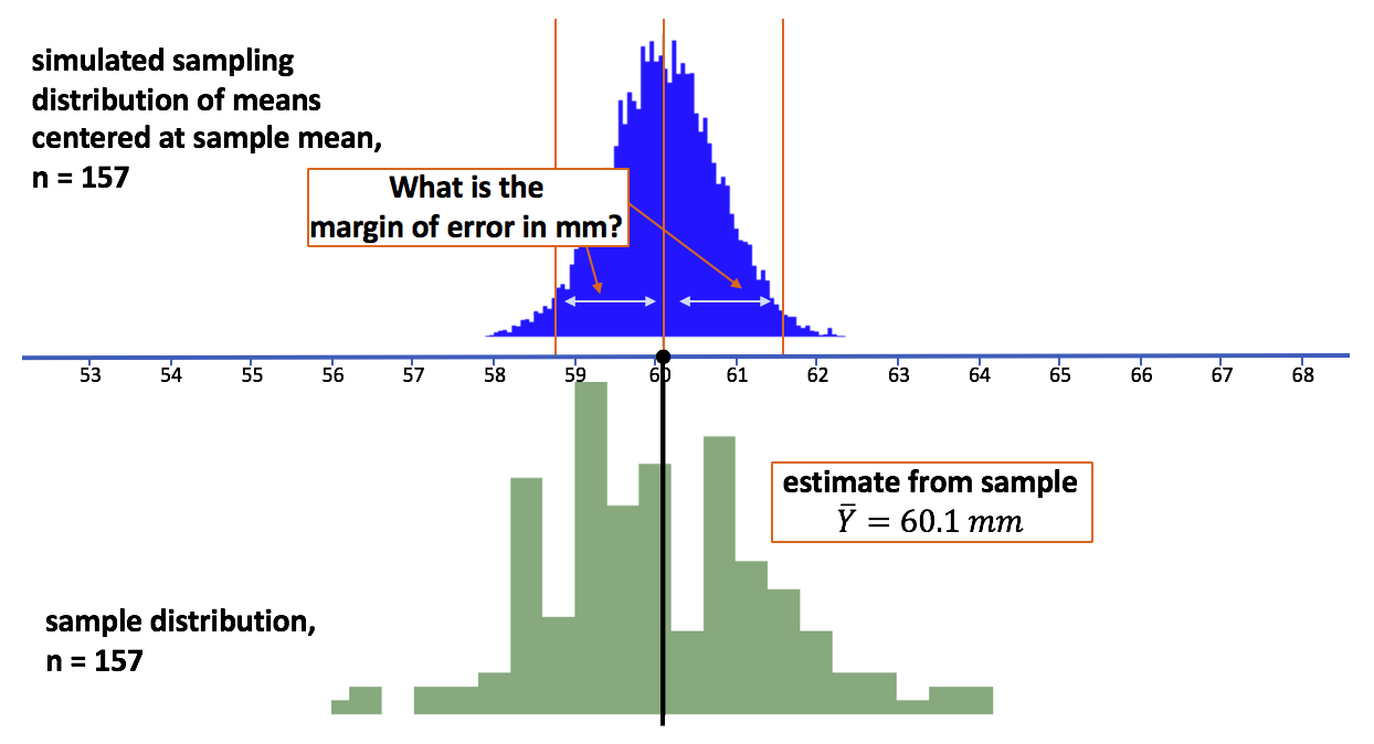
To find the margin of error, let’s find the range within which 95% of sample means would lie, assuming that \(\mu\) is 60.1. To find this range, we need to find the point below which 2.5% of simulated sample means fell, and the point above which 2.5% of simulated sample means fell.

A simple way to do this is just to arrange our 1,000 simulated means in order. Given that we simulated 1,000 means, we know that the lowest 25 means will be below the 2.5% cutoff and the highest 25 means will be above the 2.5% cutoff. These two cutoffs are located right at the lower bound and upper bound of the confidence interval.

We’ll use arrange() to put the means in simSDoM in descending order.

arrange(simSDoM, desc(mean))

Save the arranged data frame back into the same data frame, simSDoM. Then use head() and tail() to look at the first and last six lines of newly arranged data frame.

      mean
1 62.93776
2 62.38860
3 62.37687
4 62.20956
5 62.14401
6 61.98480

         mean
995  58.29070
996  58.27223
997  58.16421
998  58.04208
999  57.66940
1000 57.55213

Notice that the means are in descending order, so as you go down the column labeled mean, the numbers get smaller. If we want to find the cutoff point for the highest 2.5% of the distribution, we simply need to identify the 25th mean from the top. We will call this the upper cutoff. To find the lower cutoff, we look at the 25th mean from the bottom.

We can use the following R code to find out the 25th mean from the top.

simSDoM$mean[25] 

Type in the code to find the upper cutoff (25th mean) and the lower cutoff (976th mean).

[1] 61. 47437

[1] 58.6856

We’ve provided the code to find the margin of error from the upper cutoff to the mean. Write code to find the margin of error from the mean to the lower cutoff.

[1] 1.370703

[1] 1.408591

We find that the margin of error above the mean and below the mean is roughly 1.4 millimeters.

We know from the Central Limit Theorem that the shape of this sampling distribution is approximately normal, and thus symmetrical. We can see this in the simulated distribution of means: there seem to be as many means left of the center as right of the center. Therefore, once we find out where the lower cutoff is, we know where the upper one will be.

Constructing the Confidence Interval from the Margin of Error

We used the simulated sampling distribution centered on the sample mean in order to calculate the margin of error. It is important to remember, however, that our real interest is in the range of possible population means from which our sample could have been drawn.

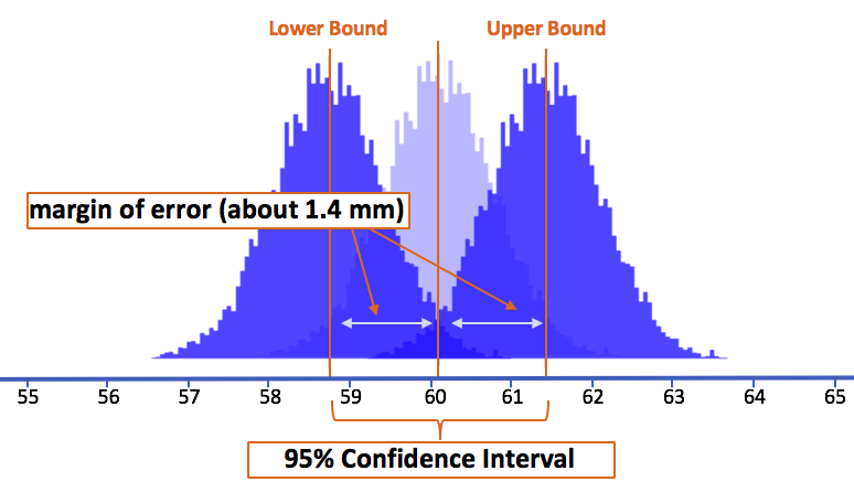
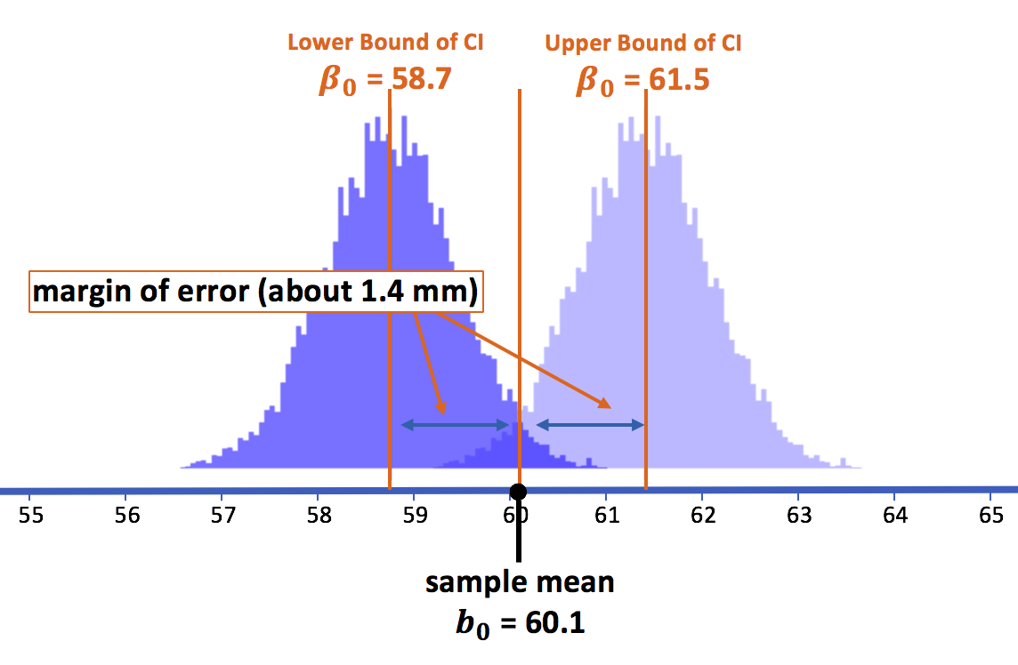
Looking again at the picture we presented earlier, we can see that the margin of error (1.4 mm) from the sample mean to each of its 2.5% tails is exactly the same distance as from the sample mean to the lower and upper bounds of the 95% confidence interval.

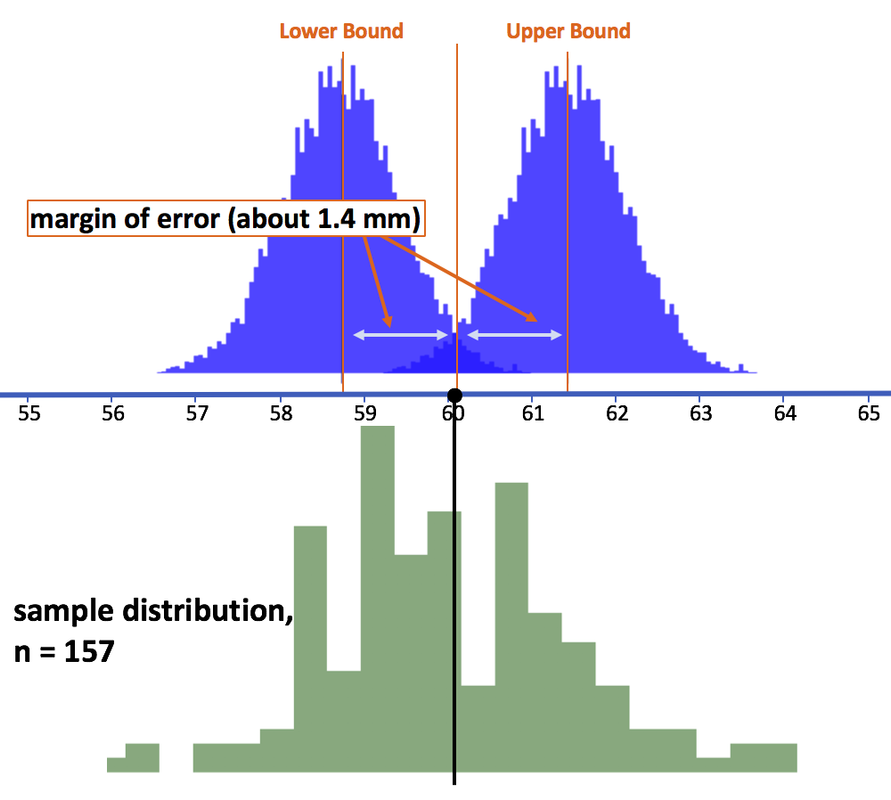
If we remove the sampling distribution centered around the sample mean from the picture, we can clearly see that the margin of error from the lower bound to its upper 2.5% cutoff ends precisely at the sample mean. And the same distance from the upper bound to its lower 2.5% cutoff also ends at the sample mean.

The key point is this: If the true population mean was at the lower bound, it means that there is only a 2.5% chance that the mean we observed (60.1 mm) or higher would have occurred had it been a random sample. And if the true population mean was at the upper bound, there is only 2.5% chance that the mean we observed or lower would have been drawn by chance.

Based on this simulation, we can say that the 95% confidence interval—the range within which we are 95% confident the true population mean must be—is 60.1 plus or minus 1.4 (or from 58.7 to 61.5). Another way of thinking of this is: this is the range of population means for which the observed mean is considered likely.

A Little Excursion to Test Our Logic

We constructed our 95% confidence interval by simulating a sampling distribution of 1,000 means, centered at our observed sample mean. But our real question was not about the tails of this distribution, but the tails of the sampling distributions that would be centered on different possible population means.

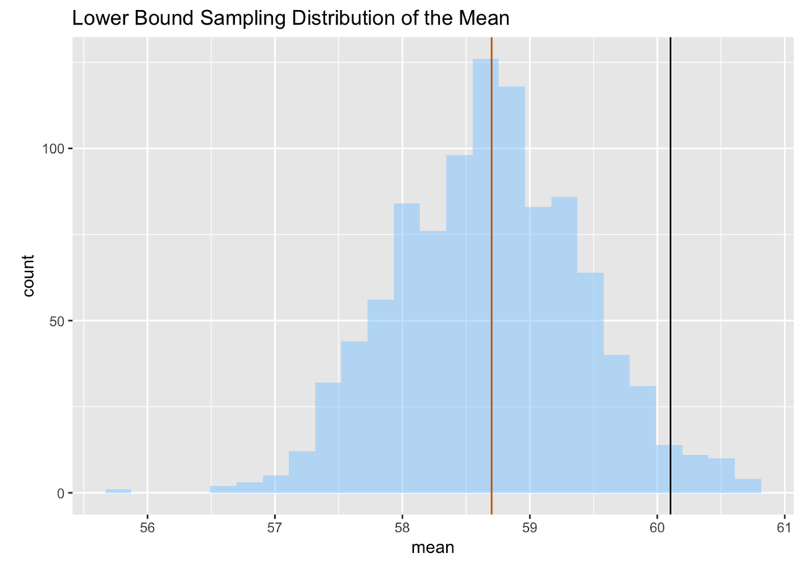
For example, if our lower boundary of the 95% confidence interval is correct, then we would reason that there would be a less than 2.5% chance of selecting a sample with a mean as high as 60.1 (the one we observed) if the true population mean were 58.7 mm (60.1 - 1.4). This makes sense logically. Let’s see if we can test it with a simulation.

Let’s use R to generate a simulation of 1,000 means from samples of 157, drawn randomly from a normally distributed population with a mean of 58.7. We’ll continue to use the standard deviation from our sample as an estimate of the population standard deviation. Plot this sampling distribution of means as a histogram and include a vertical line at the population mean (58.7) and at the sample mean (60.1).

Now the question is: where does the sample mean fall, relative to the highest 2.5% of simulated sample means? With R we can sort the scores (in descending order) and color any means higher than the 25th simulated mean (mean > mean[25]) in a different color. We’ll also include the sample mean as a vertical line.

simSDoMlower <- arrange(simSDoMlower, desc(mean))
gf_histogram(~ mean, data = simSDoMlower, fill = ~mean>mean[25], bins = 100) %>%
gf_vline(xintercept = Thumb.stats$mean)

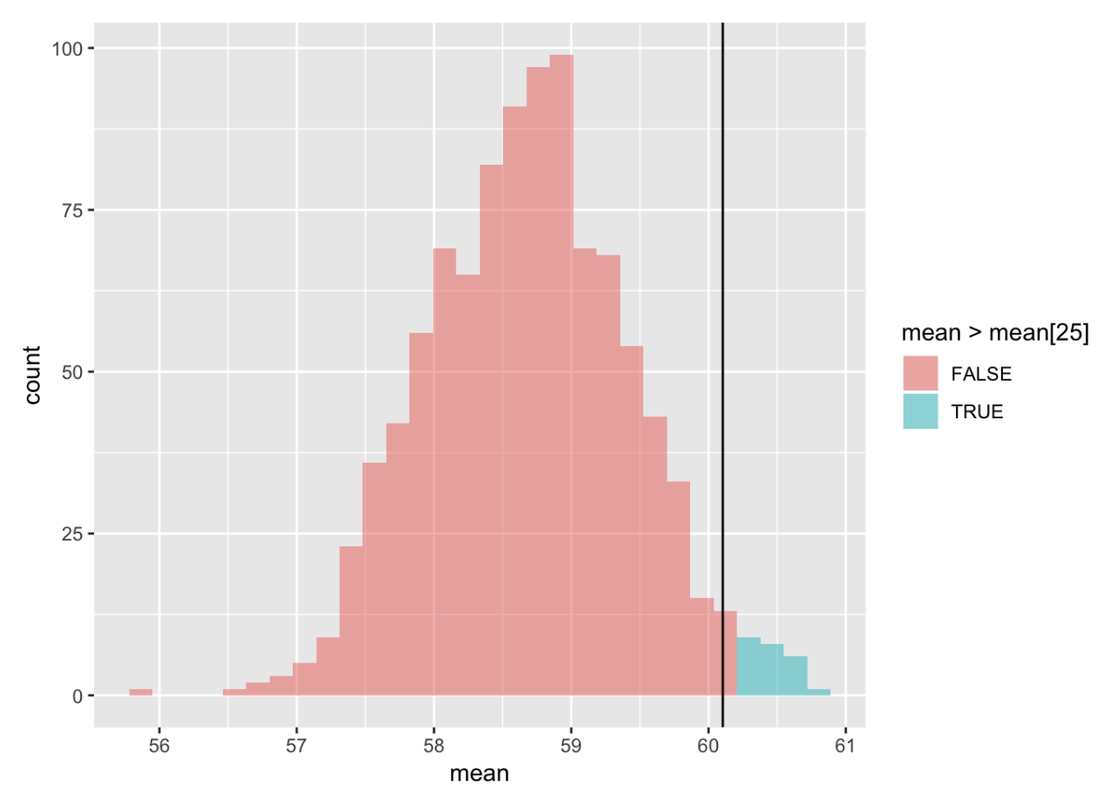
Just as we predicted, our sample mean (60.1) falls right on the upper cutoff of this sampling distribution! For reasons you may now be starting to understand, if we move our DGP and corresponding sampling distribution so that their mean is about 1.4 mm (the margin of error) to the left of our observed mean, then our sample mean becomes the upper cutoff.

We can do the same thing in the opposite direction. If we move the DGP and its simulated distribution 1.4 millimeters to the right of our sample mean (\(60.1+1.4 = 61.5\)), our sample mean would be at the cutoff point for the lower 2.5% of means that could be generated by such a DGP.

Putting all this together, we get the picture below. What it reveals is that the 95% confidence interval for the true population mean lies somewhere between -1.4 and +1.4 millimeters from the mean of our sample.

Interpreting the Simulated Confidence Interval

We have developed the argument that we can be 95% confident that the true population mean lies somewhere within our 95% confidence interval. Let’s think about what this means.

If we are 95% confident in this interval, how should we think about the other 5%? The remaining 5% is the chance of error, the chance that the interval is either too high or too low and so does not include the true population mean. If our confidence interval for the mean of thumb length is between 58.7 and 61.5, there is a 5% chance that this interval does not include true population mean (e.g. 57, or 62, or some other number).

Let’s flesh this out by thinking concretely about how we might be wrong. Again, we are using the “If…” move: What if the real population parameter was 58.5, a number slightly outside of our confidence interval?

simSDoMoutside <- do(1000) * mean(rnorm(157, mean = 58.5, sd = Thumb.stats$sd))
simSDoMoutside <- arrange(simSDoMoutside, desc(mean))
gf_histogram(~ mean, data = simSDoMoutside, fill = ~mean>mean[25]) %>%
gf_vline(xintercept = Thumb.stats$mean)  %>%
gf_labs(title = "Sampling distribution if we are wrong (population mean = 58.5)")

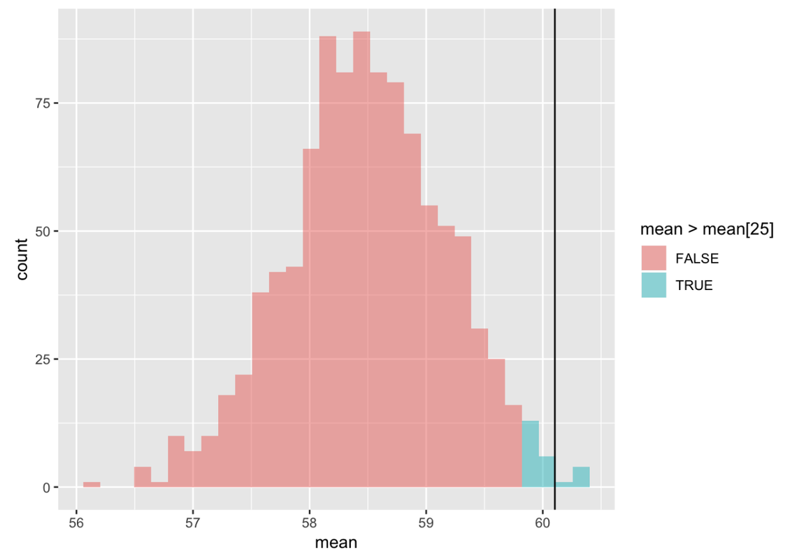
If the true population mean were 58.5, our observed mean (60.1, represented by the black line) would be slightly above the 2.5% cutoff. Could our sample have been an unlikely sample? That is, could it have been an unusually high sample mean? Yes. It will only happen 2.5% of the time, but it certainly can happen. In fact, the same process that generates the likely samples—random chance—generates the unlikely ones. It is also unlikely to roll a die 24 times and get a 6 every time, but it’s still possible. Maybe our sample was an unlikely but possible event—that the population mean was 58.5 but we happened to draw an unlikely sample. IF this is what happened and we used that sample to calculate a confidence interval, we were misled. But when it comes to confidence intervals we can be sure that they work 95% of the time.

Based on our sample, we thought the mean of the population could not be lower than the lower bound in our confidence interval, but in fact, it could be. The 95% idea keeps us aware of the fact that we might be wrong.

No Such Thing as 100% Confidence in Statistics

You might wonder: why not construct a 100% confidence interval? That way there would be a 0% chance of being wrong! Unfortunately, that is not possible; there is no such thing as 100% certainty in statistics.

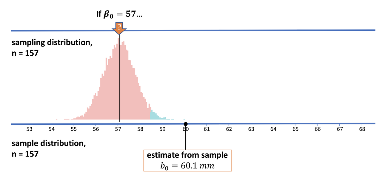
You might think that if you shift the hypothesized population mean far enough to the left (as in the picture below), there would be a 0% chance of getting a sample mean as high as 60.1. But remember, the normal distribution, which is a pretty good model of the sampling distribution of means, has tails that go on forever. While the chance of an extreme value may approach 0, it will never actually be 0.

When constructing confidence intervals we must first specify how confident we want to be in our estimate of the range of possible values of the true population mean—and 100% is not an option! A conventional starting point is 95%. But you can choose 90% or 99%, or any other number. Just not 100%.