Course Outline
-
segmentGetting Started (Don't Skip This Part)
-
segmentStatistics and Data Science: A Modeling Approach
-
segmentPART I: EXPLORING VARIATION
-
segmentChapter 1 - Welcome to Statistics: A Modeling Approach
-
segmentChapter 2 - Understanding Data
-
segmentChapter 3 - Examining Distributions
-
segmentChapter 4 - Explaining Variation
-
segmentPART II: MODELING VARIATION
-
segmentChapter 5 - A Simple Model
-
segmentChapter 6 - Quantifying Error
-
segmentChapter 7 - Adding an Explanatory Variable to the Model
-
segmentChapter 8 - Models with a Quantitative Explanatory Variable
-
8.4 Examining Residuals from the Model
-
segmentPART III: EVALUATING MODELS
-
segmentChapter 9 - Distributions of Estimates
-
segmentChapter 10 - Confidence Intervals and Their Uses
-
segmentChapter 11 - Model Comparison with the F Ratio
-
segmentChapter 12 - What You Have Learned
-
segmentFinishing Up (Don't Skip This Part!)
-
segmentResources
list full book
8.4 Examining Residuals From the Model
Now you’re on a roll! You probably remember from the previous chapter how to save the residuals from a model. We can do the same thing with a regression model: whenever we fit a model, we can generate both predictions and residuals from the model.
Try to generate the residuals from the Height.model that you fit to the full Fingers data set.
            require(tidyverse)
            require(mosaic)
            require(Lock5Data)
            require(supernova)

            Fingers <- filter(Fingers, Thumb >= 33 & Thumb <= 100)
            Height.model <- lm(Thumb ~ Height, data = Fingers)
            # modify to save the residuals from Height.model
            Fingers$Height.resid <- resid()
            # modify to save the residuals from Height.model
            Fingers$Height.resid <- resid(Height.model)
ex() %>% check_object("Fingers") %>% check_column("Height.resid") %>% check_equal()
            require(tidyverse)
            require(mosaic)
            require(Lock5Data)
            require(supernova)

            Fingers <- filter(Fingers, Thumb >= 33 & Thumb <= 100)
            Height.model <- lm(Thumb ~ Height, data = Fingers)
            Fingers$Height.resid <- resid(Height.model)
            # modify to make a histogram of Height.resid
            gf_histogram()
gf_histogram(~Height.resid, data = Fingers)
            ex() %>% {
                check_function(., "gf_histogram") %>%
                    check_arg("object") %>%
                    check_equal(incorrect_msg = "Did you remember to use ~Height.resid in the first argument?")
                check_function(., "gf_histogram") %>%
                    check_arg("data") %>%
                    check_equal(incorrect_msg = "Make sure to set data = Fingers")
            }
~ means "as a function of"
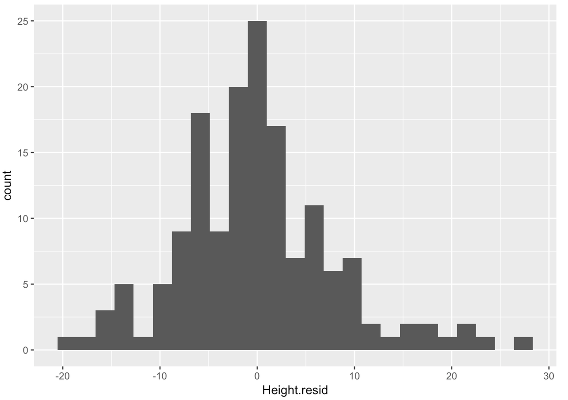
The residuals from the regression line are centered at 0, just as they were from the empty model, the two-group model, and the three-group model. In those previous models, this was true by definition: deviations of scores around the mean will always sum to 0 because the mean is the balancing point of the residuals. Thus the sum of these negative and positive residuals will be 0.
It turns out this is also true of the best-fitting regression line: the sum of the residuals from each score to the regression line add up to 0, by definition. In this sense, too, the regression line is similar to the mean of a distribution in that it perfectly balances the scores above and below the line.