9.1 Exploring the Variation in an Estimate
To explore the concept of variation in estimates, let’s go back to an example we explored in Chapter 3: the throwing of a die. We start there because we know the DGP, and because we know what it is, we can investigate the variation across samples using simulation techniques.
We know, and we confirmed earlier, that in the long run a population of die rolls has a uniform distribution. If we roll a die one time, we don’t know if it will come out a 1, 2, 3, 4, 5, or 6. But if we throw a die 10,000 times (or throw 10,000 dice all at the same time), we should end up with a uniform distribution. Note that we just picked 10,000 as a really big number but it could have been any big number (e.g., 100,000 or 259,240 or 17,821, etc).
Using the resample() function, we simulated 10,000 die rolls.
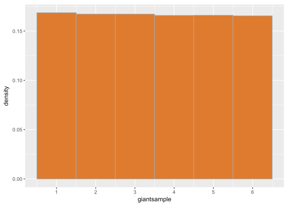
giantsample <- resample(1:6, 10000)Then we plotted this distribution in a histogram (below). You can see that the distribution is almost perfectly uniform, as we would expect. But it’s not perfect; there is some tiny variation across the six possible outcomes.
We learned in Chapter 3, though, that if we take a smaller sample of die rolls (let’s say n=24), we get a lot more variation among samples. And, perhaps most important, none of them look so much like the population.
Here’s code we used to randomly generate a sample of n=24 die rolls.
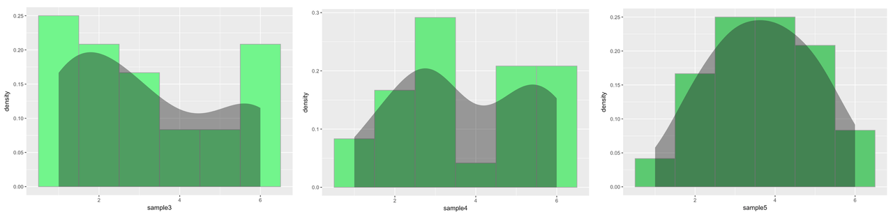
sample <- resample(1:6, 24)Each time we ran this function, we got a different looking distribution. Here are a few samples of 24 die rolls. (We put density plots on them so you could appreciate how different the overall shapes were.)
From Sample to Estimate
Up to this point we have discussed sampling variation in a qualitative way. We can see that the samples are different, and also that none of them look very much like what we know the population looks like.
But now we want to go further. Imagine that we didn’t know the DGP of this distribution, and we were analyzing one sample in order to find out.
We know a lot more about how to do this than we did in Chapter 3! Use the code window to generate a sample of n=24 die rolls and save it as sample1. We’ve added additional code to print out the 24 numbers that result and then calculate the mean of the 24 numbers (our parameter estimate).
            require(tidyverse)
            require(mosaic)
            require(Lock5Data)
            require(supernova)

            RBackend::custom_seed(4)
            # Write code to simulate a random sample of 24 die rolls
            sample1 <-

            # This will print the 24 numbers in sample1
            sample1

            # This will return the mean of these numbers
            mean(sample1)
            # Write code to simulate a random sample of 24 die rolls
            sample1 <- resample(1:6, 24)

            # This will print the 24 numbers in sample1
            sample1

            # This will return the mean of these numbers
            mean(sample1)
            ex() %>% {
                check_function(., "resample") %>% check_arg("...") %>% check_equal()
                check_output_expr(., "sample1")
                check_function(., "mean") %>% check_result() %>% check_equal()
            }
resample will draw randomly from the same set of numbers with replacement[1] 4 1 2 2 5 2 5 6 6 1 5 2 1 6 3 3 6 4 6 5 5 6 4 3[1] 3.875Our sample of n=24 had a mean of 3.875. (Note: In your code window, you may have gotten a different sample mean because your random sample was different from ours.) If this were our only sample, we’d use 3.875 as our best estimate of the population mean. But because we know what the DGP looks like, we can know, in this case, what the mean of the population should be.
Let’s calculate the expected mean in two ways. First, let’s simulate 10,000 die rolls like we did above, and then calculate their mean. Modify the code in the code window to do this.
            require(tidyverse)
            require(mosaic)
            require(Lock5Data)
            require(supernova)

            RBackend::custom_seed(10)
            # Generate a giant sample of 10000 die rolls
            giantsample <- resample()

            # Calculate the mean of the giant sample
            # Generate a giant sample of 10000 die rolls
            giantsample <- resample(1:6, 10000)

            # Calculate the mean of the giant sample
            mean(giantsample)
            ex() %>% {
                check_function(., "resample") %>% check_arg("...") %>% check_equal()
                check_function(., "mean") %>% check_result() %>% check_equal()
            }
Here’s what we got for the mean of our giant sample of 10,000:
[1] 3.48957It’s very close to 3.5. Another way to get the expected mean is just to calculate the mean of each of the equally likely outcomes of a die roll: 1, 2, 3, 4, 5, 6. Use the code window below to do this.
            require(tidyverse)
            require(mosaic)
            require(Lock5Data)
            require(supernova)
            # These are the possible outcomes of a die roll.
            die_outcomes <- c(1, 2, 3, 4, 5, 6)

            # Modify this code to find the mean of the possible outcomes
            mean()
            # These are the possible outcomes of a dice roll.
            die_outcomes <- c(1, 2, 3, 4, 5, 6)

            # Modify this code to find the mean of the possible outcomes
            mean(die_outcomes)
ex() %>% check_function("mean") %>% check_result() %>% check_equal()
[1] 3.5Now you get exactly 3.5, which is what the population mean should be. It’s the exact middle of the numbers 1 to 6, and if each is equally likely, 3.5 would have to be the mean.
But then let’s remember our small sample (sample1, n=24)—the mean was 3.875. Because we know the true population mean is 3.5, it’s easy in this case to quantify how different our sample is from the true mean of the population: the difference is 3.875—3.5 (or .375).
Let’s try it. It’s easy enough to simulate another random sample of n=24. Let’s save it as sample2 and see what the mean is.
            require(tidyverse)
            require(mosaic)
            require(Lock5Data)
            require(supernova)
            RBackend::custom_seed(12)
            # Write code to simulate another random sample of 24 dice rolls
            sample2 <-

            # This will return the mean of those numbers
            mean(sample2)
            # Write code to simulate another random sample of 24 dice rolls
            sample2 <- resample(1:6, 24)

            # This will retrn the mean of those numbers
            mean(sample2)
            ex() %>% {
                check_function(., "resample") %>% check_arg("...") %>% check_equal()
                check_function(., "mean") %>% check_result() %>% check_equal()
            }
[1] 2.875We know, in this case, that the mean of the population is 3.5. But if we were trying to estimate the mean based on our samples, we would have a problem. The two random samples of n=24 we have generated so far produced two different estimates of the population mean: 3.875 and 2.875 (sample1 and sample2, respectively).
Let’s look at a few more samples. But let’s not bother saving the result of each die roll in each sample. Instead, let’s just simulate a random sample of 24 die rolls and calculate the mean, all in one line of R code.
mean(resample(1:6, 24))Try running the code to see what the mean is for a third random sample of 24 die rolls.
            require(tidyverse)
            require(mosaic)
            require(Lock5Data)
            require(supernova)
            RBackend::custom_seed(13)
            # run this code
            mean(resample(1:6, 24))
           # run this code
            mean(resample(1:6, 24))
ex() %>% check_error()
[1] 3.166667So far we have generated a diverse group of sample means, and no two are alike: 3.875, 2.875, 3.167.
This line of reasoning starts to raise this question in our minds: Are some sample means more likely than others?