3.5 The Back and Forth Between Data and the DGP (Continued)

Examining Variation Across Samples

Let’s take a simulated sample of 12 die rolls (sampling with replacement from the six possible outcomes) and save it in a vector called sample1.

Then let’s save that vector as a variable in a data frame called dicerolls.

dicerolls <- data.frame(sample1)

This creates a data frame called dicerolls with a single variable in it called sample1. It might seem like overkill to make a data frame for just one variable, but there are things we can do with a data frame–e.g., make graphs using the ggformula functions–that we can’t do with just a vector. And once we have a data frame, we can keep adding new variables (i.e., columns) to it.

For example, gf_histogram() always expects a ~, then a variable, then data = followed by the name of a data frame. You can imagine variables inside a data frame as like rooms inside of a building. In this case, there is just one room (sample1) inside the building (dicerolls).

Add some code to create a density histogram (which could also be called a relative frequency histogram) to examine the distribution of our sample. Set bins=6.

Your random sample will look different from ours (after all, random samples differ from one another) but here is one of the random samples we generated.

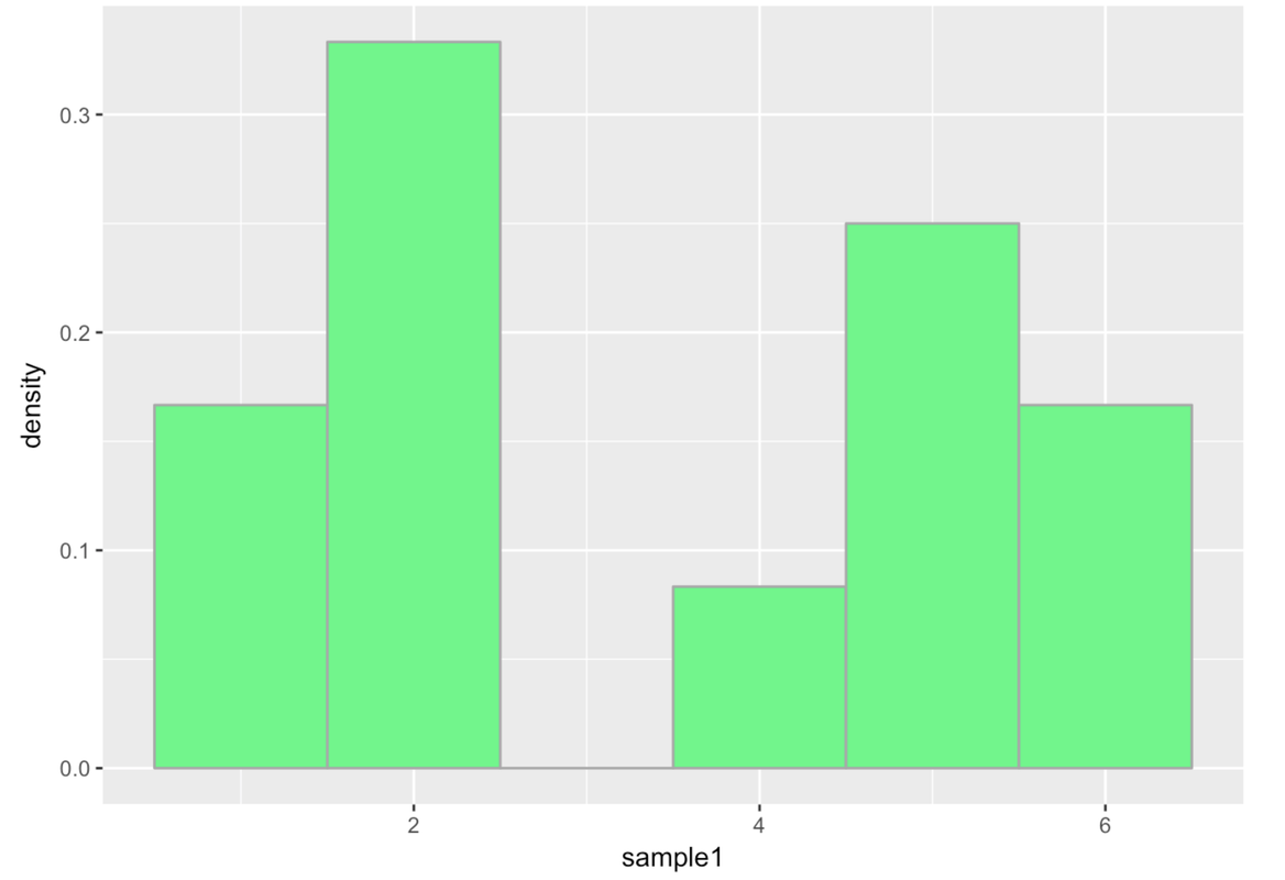
(Just a reminder–our histograms may look different because we might fancy up our histograms with colors and labels and things. Sometimes we may ask you to refrain from doing so because it makes it harder for R to check your answer.) Notice that this doesn’t look very much like the uniform distribution we would expect based on our knowledge of the DGP!

Let’s take a larger sample—24 die rolls. Modify the code below to simulate 24 die rolls, save it as a vector called sample2, and then put this vector in a data frame. Will the distribution of this sample be perfectly uniform?

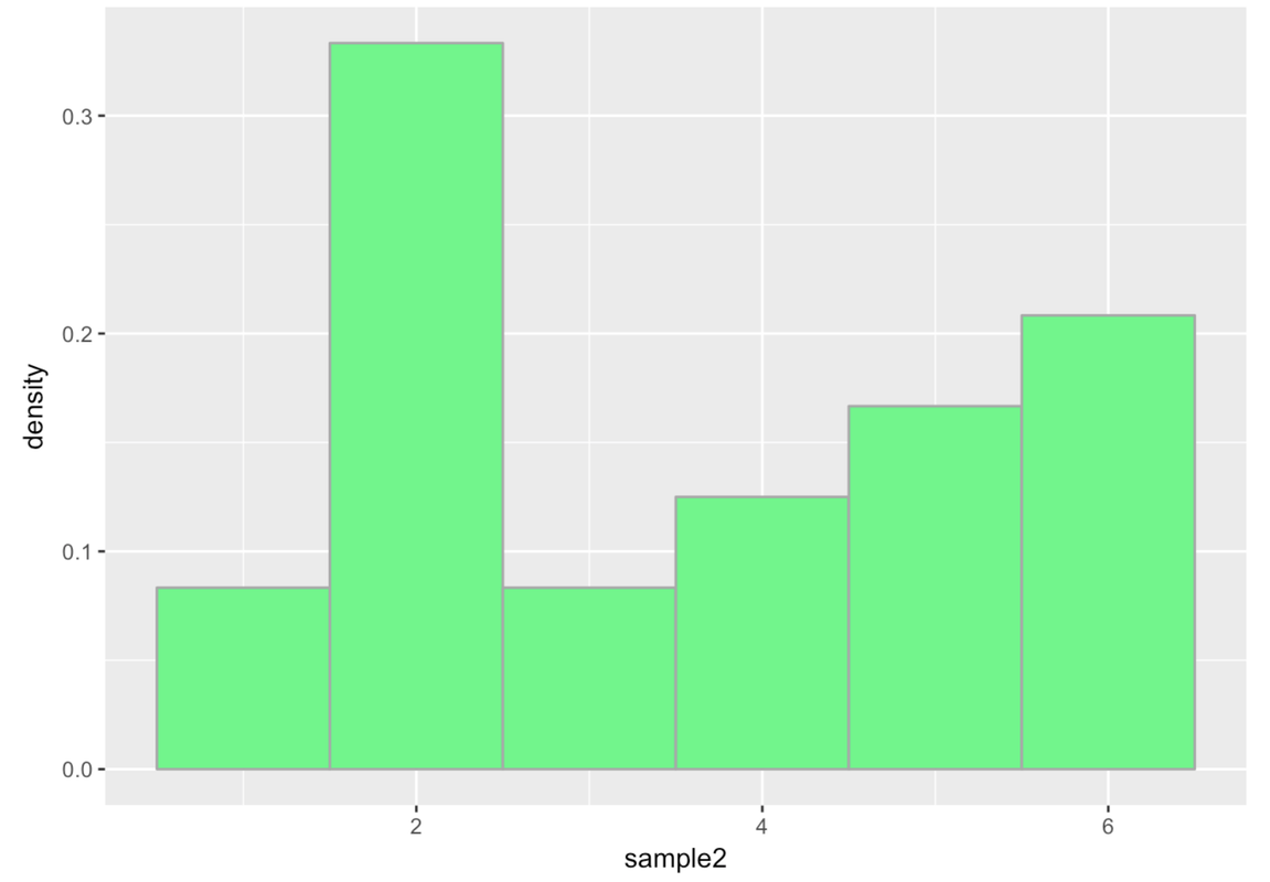
Notice that our randomly generated sample distribution is also not perfectly uniform. In fact, this doesn’t look very uniform to our eyes at all! You might even be asking yourself, is this really a random process?

Simulate a few more samples of 24 die rolls (we will call them sample3, sample4, and sample5) and plot them on histograms. This time, add a density plot on top of your histograms (using gf_density()). Do any of these look exactly uniform?

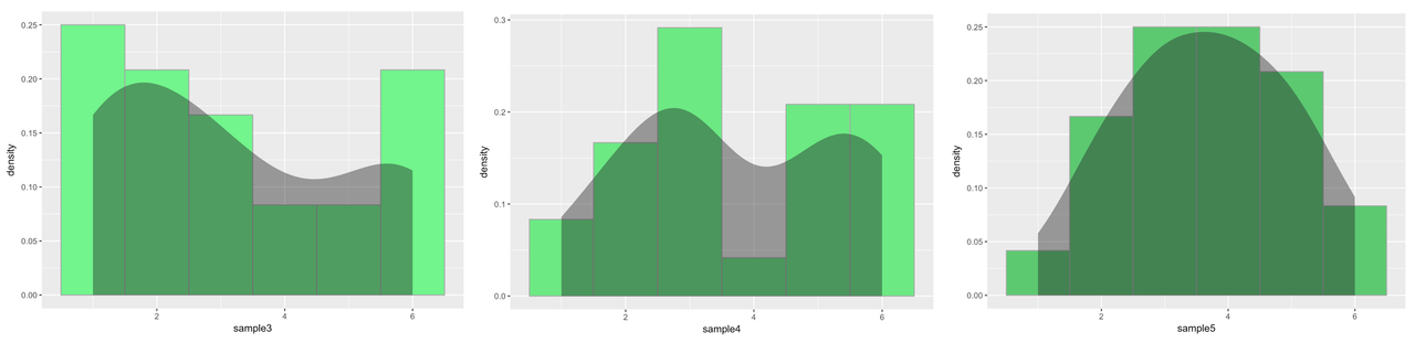
Wow, these look crazy and they certainly do not look uniform. They also don’t even look similar to each other. What is going on here?

The fact is, these samples were, indeed, generated by a random process: simulated die rolls. And we assure you, at least here, there is no error in the programming. The important point to understand is that sample distributions can vary, even a lot, from the underlying population distribution from which they are drawn. This is what we call sampling variation. Small samples will not necessarily look like the population they are drawn from, even if they are randomly drawn.

Large Samples Versus Small Samples

Even though small samples will often look really different from the population they were drawn from, larger samples usually will not.

For example, if we ramped up the number of die rolls to 1,000, we will see a more uniform distribution. Complete then run the code below to see.

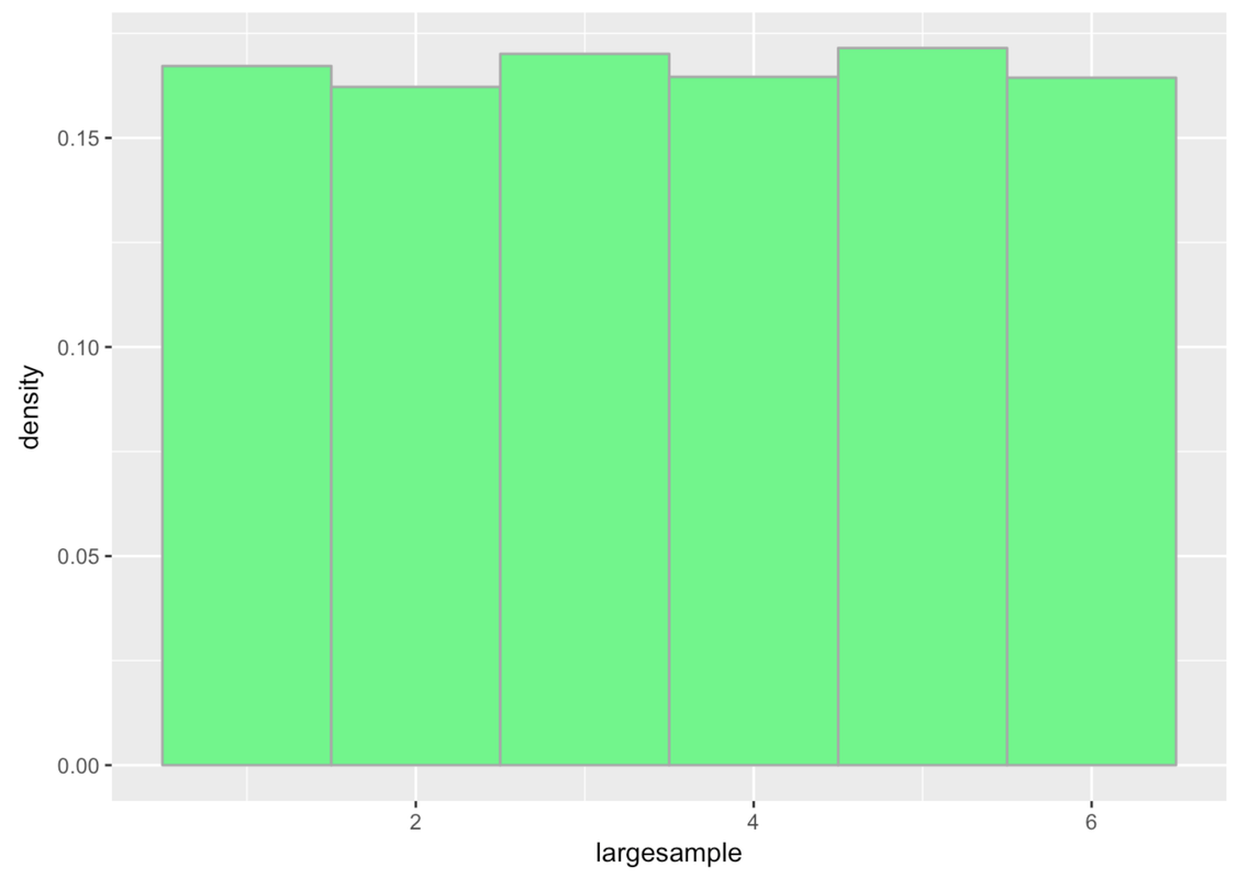
Wow, a large sample looks a lot more like what we expect the distribution of die rolls to look like! This is also why we make a distinction between the DGP and the population. When you run a DGP (such as resampling from the numbers 1 to 6) for a long time (like 10,000 times), you end up with a distribution that we can start to call a population.

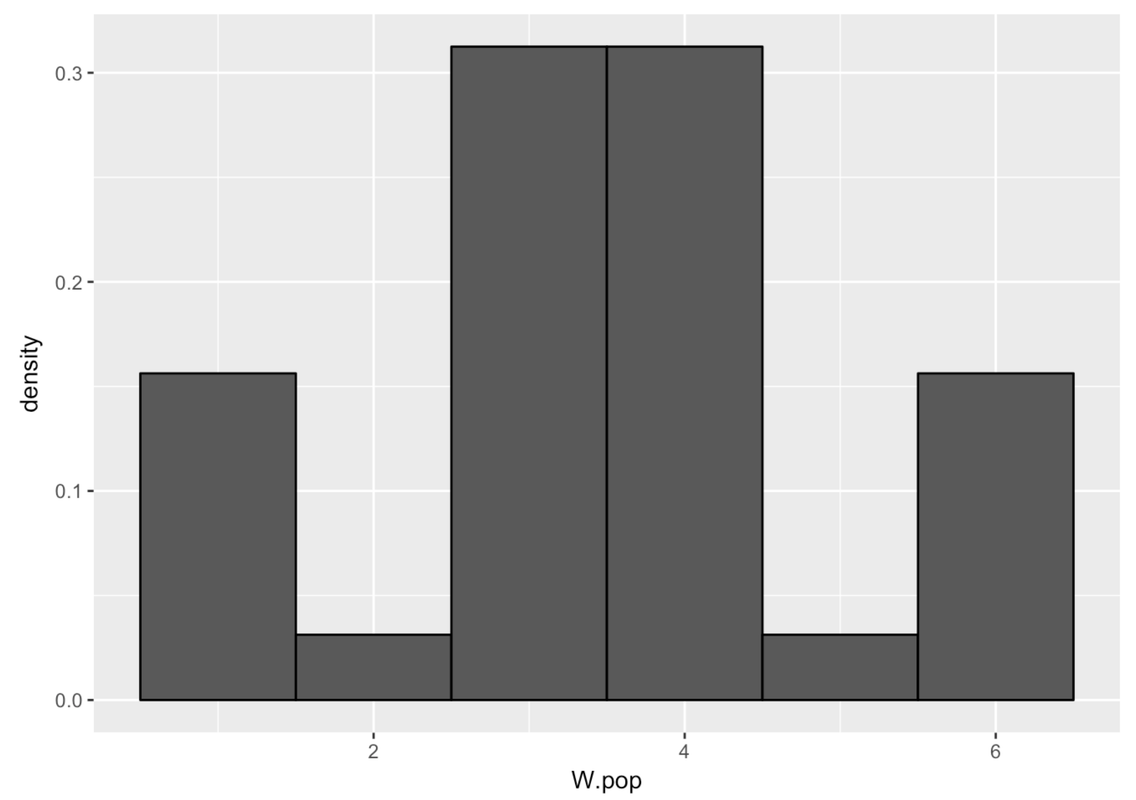
Even though small samples are unreliable and sometimes misleading, large samples usually tend to look like the parent population that they were drawn from. This is true even when you have a weird population. For example, we made up a simulated population that kind of has a “W” shape. We put it in a variable called W.pop (it’s in the weird data frame). Here’s a density histogram of the population.

gf_dhistogram( ~ W.pop, data = weird, color = "black", bins = 6)

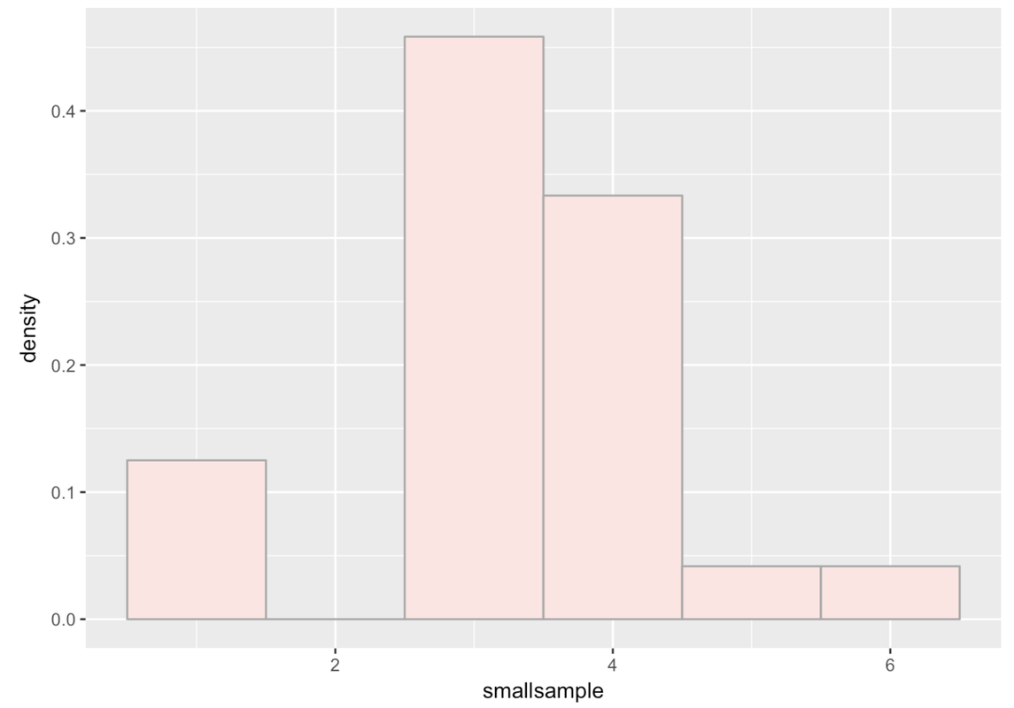
Now try drawing a relatively small sample (n = 24) from W.pop (with replacement) and save it as smallsample. Put your small sample in the weird data frame. Let’s observe whether the small sample looks like this weird W-shape.

Now try drawing a large sample (n = 1,000) and save it as largesample. Will this one look more like the weird population it came from than the small sample?

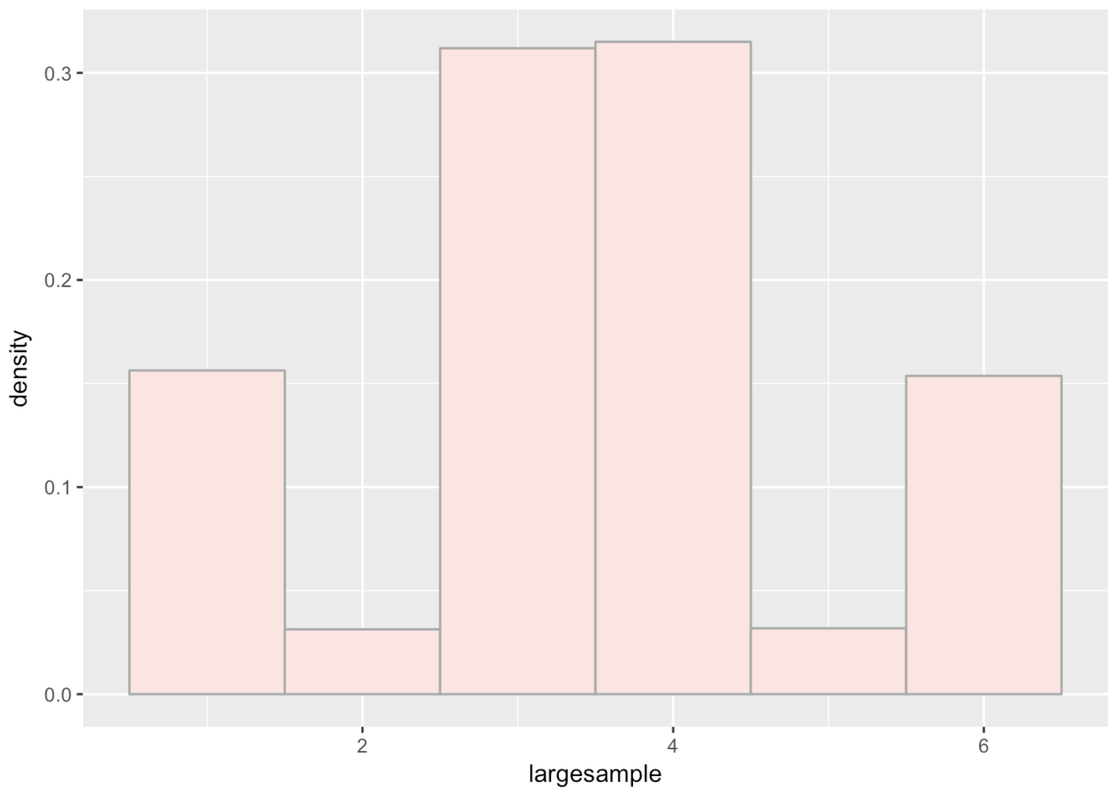
That looks very close to the W-shape of the simulated population we started off with.

This pattern that large samples tend to look like the populations they came from is so reliable in statistics that it is referred to as a law: the law of large numbers. This law says that, in the long run, by either collecting lots of data or doing a study many times, we will get closer to understanding the true population and DGP.

Lessons Learned

In the case of dice rolls (or even in the weird W-shaped population), we know what the true DGP looks like because we made it up ourselves. Then we generated random samples. What we learned is that smaller samples will vary, with very few of them looking exactly like the process that we know generated them. But a very large sample will look more like the population.

In fact, it is unusual in real research to know what the true DGP looks like. Also we rarely have the opportunity to collect truly large samples! In the typical case, we only have access to relatively small sample distributions, and usually only one sample distribution. The realities of sampling variation, which you have now seen up close, make our job very challenging. It means we cannot just look at a sample distribution and infer, with confidence, what the parent population and DGP look like.

On the other hand, if we think we have a good guess as to what the DGP looks like, we shouldn’t be too quick to give up our theory just because the sample distribution doesn’t appear to support it. In the case of die rolls, this is easy advice to take: even if something really unlikely happens in a sample—e.g., 24 die rolls in a row all come up 5—we will probably stick with our theory! After all, a 5 coming up 24 times in a row is still possible to occur by random chance, although very unlikely.

But when we are dealing with real-life variables, variables for which the true DGP is fuzzy and unknown, it is more difficult to know if we should dismiss a sample as mere sampling variation just because the sample is not consistent with our theory. In these cases, it is important that we have a way to look at our sample distribution and ask: how reasonable is it to assume that our data could have been generated by our current theory of the DGP?

Simulations can be really helpful in this regard. By looking at what a variety of random samples look like, we can get a sense as to whether our particular sample looks like natural variation, or if, instead, it sticks out as wildly different. If the latter, we may need to revise our understanding of the DGP.