11.2 Sampling Distribution of PRE and F

A Sampling Distribution of PRE

As it turns out, we can construct a sampling distribution of any statistic we calculate from our sample, including our estimate of PRE. We are also going to introduce a new function called PRE(). This function gives us another way to calculate PRE from our sample.

PRE(Tip ~ Condition, data = TipExperiment)

We can also save this PRE in an R object (we’ll just call it samplePRE). Write some code to print out the samplePRE. Try running all of it in the code window below.

[1] 0.07294944

Notice that we just get the same PRE we got in the ANOVA table (from the function supernova()).

Now we will we use our “If…” thinking to imagine a DGP with no relationship between Condition and Tip. The shuffle() function will help us break whatever relationship exists between these two variables. This technique is sometimes called randomization (it is also sometimes called the permutation approach).

Below is the R code necessary to calculate the PRE of the Condition model for one shuffled (or randomized) set of data. This code will 1) shuffle around the values of Condition, 2) create a model of Tip using Condition as an explanatory variable, then 3) calculate the PRE of that complex model.

PRE(Tip ~ shuffle(Condition), data = TipExperiment)

Modify the code written in the code window below to include the idea of “shuffling the values of Condition.”

[1] 0.000202076

We got a very small PRE when we shuffled the values of Condition around.

Now let’s extend this code with the function do() to simulate 1,000 PREs. Modify the bit of code in the code window to calculate 1,000 PREs from randomized data. Save them into a data frame called SDoPRE (Sampling Distribution of PREs).

          PRE
1 0.064437507
2 0.068627491
3 0.003963164
4 0.003006396
5 0.023197503
6 0.001488764

This code is using a randomization process to generate the sampling distribution. It starts with the data points collected by the researchers, but then reassigns each data point to a random group (Smiley Face or Control).

Up to this point, it’s very similar to the process we used above to create a sampling distribution of the differences of means. But this time, once we create the two simulated groups, instead of calculating their means and taking the difference, we fit the linear model and calculate PRE. And, we do this 1,000 times.

The resulting sampling distribution is plotted in the histogram below. We’ve also printed out the favstats.

gf_histogram(~ PRE, data = SDoPRE, fill = "orange", alpha = .0)
favstats(~ PRE, data = SDoPRE)

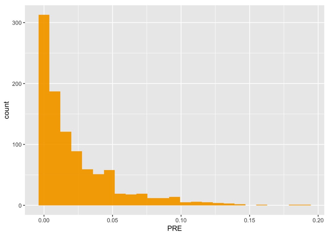
       min          Q1     median         Q3       max       mean         sd    n missing
 4.124e-06 0.003006396 0.01202971 0.03266621 0.1906319 0.02289922 0.02854204 1000       0

The shape of this sampling distribution of PRE is quite different from the sampling of means or of the differences between means. It is bunched up on the left, with a long tail on the right.

If a sampling distribution was normally distributed, we would calculate the probabilities in each of the two tails, adding them up to get the overall probability of a score or mean or mean difference as extreme as the one we observed. With the sampling distribution of PRE, we only need to look at one tail of the distribution. We know that PRE can never be less than 0. We just want to know how likely it is to get a PRE as high as the one we observed.

In the Tipping study, the researchers observed a sample PRE of .0729. See if you can modify the histogram to color the PREs that are greater than the sample PRE in a different color. Also, find the proportion of the 1,000 randomized PREs in the sampling distribution that are greater than our sample PRE, .0729. Use the code window below (where we have already entered the code to save the samplePRE, and create the sampling distribution in the data frame SDoPRE).

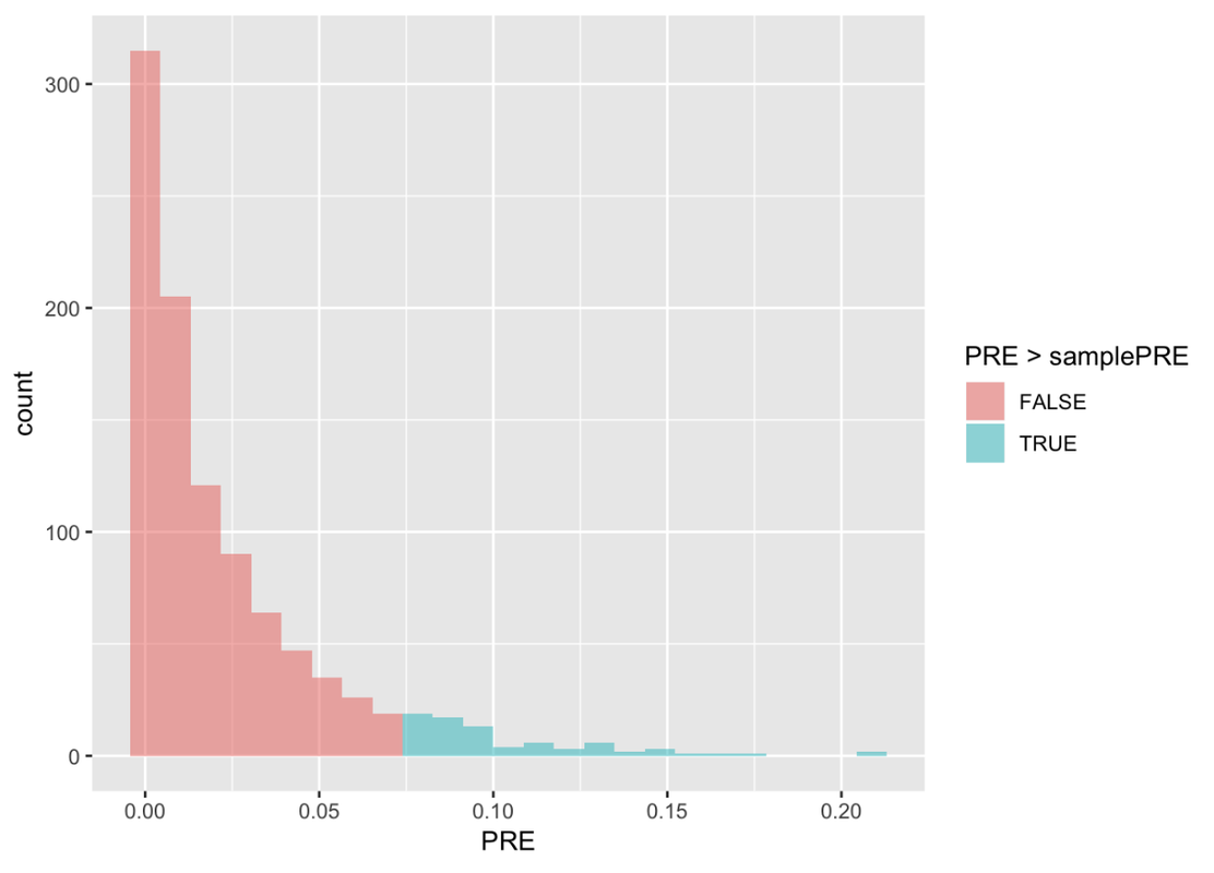
PRE > samplePRE
 TRUE FALSE 
0.078 0.922

In our sampling distribution, only .078 (or about .08) of the randomized samples had PREs greater than our sample PRE.

Randomization is a DGP that makes any difference between group means meaningless. This DGP is emulating a world where the true PRE is actually 0. This sampling distribution of PREs shows us that even if the true DGP were a PRE of 0, there would still be a .08 chance of obtaining the observed difference between the Smiley Face and Control groups. So, just like before, because there is a greater than .05 chance that the observed difference could have been obtained just by chance, we will not reject the simple (or empty) model.

A Sampling Distribution of F

Let’s try the same approach, but this time let’s simulate a sampling distribution of F ratios instead of PREs.

First, let’s save our sample F as an R object using a new function called fVal().

sampleF <- fVal(Tip ~ Condition, data = TipExperiment)

Try printing out the sampleF in the code window.

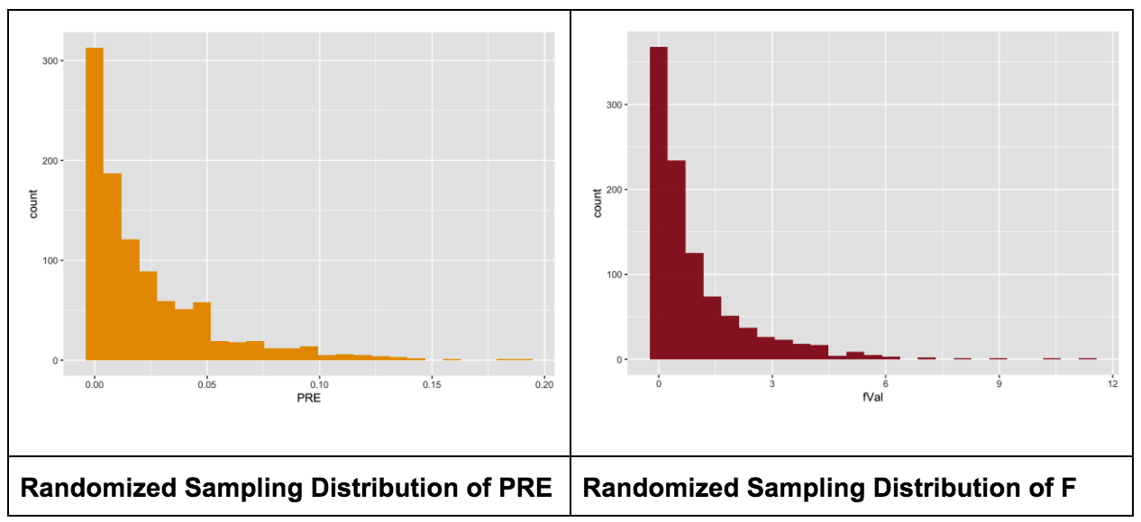
[1] 3.304973

Like we did with the sampling distribution of PRE, we are going to imagine the same DGP where any difference between groups is just due to randomization. Here is the code for randomizing the same data 1,000 times, but this time saving the F values in a sampling distribution, and then plotting a histogram of the sampling distribution.

SDoF  <-  do(1000) * fVal(Tip ~ shuffle(Condition), data = TipExperiment)
gf_histogram(~ fVal, data = SDoF, fill = "firebrick", alpha = .9)

We display a histogram of the simulated sampling distribution of F (right) next to the one for PRE (left) so that you can compare them.

The sample F observed in the actual study was 3.305. In the code window, modify the histogram to color the fVals that are greater than the sample F in a different color. Also, find the proportion of the 1,000 randomized Fs in the sampling distribution that are greater than our sample F. What do you think this proportion will be?

Use the code window below (where we have already entered the code to save the sampleF), and create the sampling distribution in the data frame SDoF.

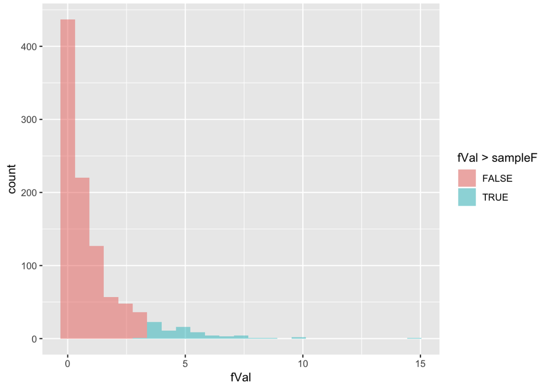
fVal > sampleF
 TRUE FALSE 
0.076 0.924

 Analysis of Variance Table
 Outcome variable: Tip
 Model: [1] "Tip ~ Condition"
 
                               SS df     M S     F    PRE     p
 ----- ----------------- -------- -- ------- ----- ------ -----
 Model (error reduced) |  402.023  1 402.023 3.305 0.0729 .0762
 Error (from model)    | 5108.955 42 121.642                   
 ----- ----------------- -------- -- ------- ----- ------ -----
 Total (empty model)   | 5510.977 43 128.162

In the table below we have pasted in the supernova(Condition.model) result again. The PRE was .0729. The F was 3.305. We can use tally() to calculate the number of randomized samples with F ratios greater than 3.305 (out of 1000) just as we did for PRE. We have put the results below, again for both our randomized sampling distributions of PRE and F.

Analysis of Variance Table
 Outcome variable: Tip
 Model: lm(formula = Tip ~ Condition, data = TipExperiment)
 
                              SS df     MS     F    PRE     p
 ----- ----------------- ------- -- ------ ----- ------ -----
 Model (error reduced) |  402.02  1 402.02 3.305 0.0729 .0762
 Error (from model)    | 5108.95 42 121.64                   
 ----- ----------------- ------- -- ------ ----- ------ -----
 Total (empty model)   | 5510.98 43 128.16

PRE > samplePRE
 TRUE FALSE 
0.078 0.922

fVal > sampleF
 TRUE FALSE 
0.076 0.924

As you can see, we get almost exactly the same results: .08 out of 1,000 randomized samples have Fs greater than the observed F, compared with .08 of 1,000 randomized PREs. This value corresponds to the “p” column at the very end of the ANOVA table (.0762). This is often called the p-value.

When you think about the p-value, we want you to think about the process that got us here. We imagined and implemented a DGP where the explanatory variable did not matter (also called the empty model or null hypothesis). This DGP produced a sampling distribution of a statistic (e.g., PRE or F ratio). The p-value is the likelihood that a value more extreme than our sample statistic would be generated from the empty model.

A probability of .05 (or 5%) or less is defined as “unlikely” by cultural convention: the community of statistics users agreed on this. A small p-value (e.g., ≤ .05) indicates that our statistic is unlikely to have been generated by the empty model so we would reject this model of the DGP. Conversely, a large p-value (e.g., > .05) indicates that our statistic could have been generated by the empty model, so you fail to reject it.