10.7 Using Confidence Intervals to Evaluate a Group Difference

Up to this point we have used confidence intervals to estimate the range of possible values for the population mean (or, if we are using the empty model, \(\beta_0\)). But confidence intervals can also be constructed around other parameters—often parameters that we care more about.

Let’s return to the two-group model that we developed in Chapter 7. Recall that we constructed a variable with two levels, Height2Group, that divided our sample into two groups, Short and Tall. We were investigating whether some of the variation in thumb length might be explained by which height group a person was in.

We fit the Height2Group model using the following R code:

Height2Group.model <- lm(Thumb ~ Height2Group, data = Fingers)
Height2Group.model

Here is the model fit that resulted:

Call:
lm(formula = Thumb ~ Height2Group, data = Fingers)

Coefficients:
     (Intercept)  Height2Grouptall
          57.818             4.601

The two-group model we fit can be represented like this in the notation of the General Linear Model:

\[Y_{i}=b_{0}+b_{1}X_{i}+e_{i}\]

Recall that \(X_i\) would take the value 0 for people categorized as Short, and 1 for those deemed Tall. So, the parameter estimate \(b_1\) represents the observed magnitude of the difference in mean thumb lengths between the two groups.

Why We Would Want a Confidence Interval

We can construct a confidence interval for our estimate of \(\beta_1\) using the same method we used previously to get a confidence interval around the mean. Before we construct that confidence interval, though, it is useful to think about why we would want one.

Although the researchers observed a difference in means between the two groups (Short and Tall), it’s possible that the difference was simply due to sampling variation. If we did our thumb length and height group study with another group of 157 students, we would come up with different estimates, \(b_{0}\) and \(b_{1}\). What we really want to know is, what is the true difference in means (\(\beta_1\)) between the two groups in the population?

Let’s do a little thought experiment to help us see why this is important. What if we have samples from two groups (just as we do here), but we know for a fact that the two populations have identical means? In other words, we know that the true value of \(\beta_1\) is 0. If we take multiple samples from these two populations, we will get various estimates of the group difference. Importantly, although the estimates would be expected to cluster around 0, we now know for a fact that they would vary; the chance of getting a mean difference of exactly 0 would be relatively small.

By constructing a confidence interval for our estimate of \(b_1\) we can see whether, despite an observed difference in means, it is possible that the true difference in means is 0. In a two-group comparison, this is generally what we want to know: is the observed difference between the two groups real, or could it just have occurred as a consequence of sampling variation? And if there is a real difference, how big could the difference be? The confidence interval can answer both of these questions.

Constructing a Bootstrapped Sampling Distribution of \(b_{1}\)

To construct a confidence interval around our parameter estimate \(b_{1}\), we first need to construct a sampling distribution of the estimate. Once we have that, we can use it to find the upper and lower boundaries for the 95% confidence interval around the parameter estimate.

We know from the lm() model fit above that our sample estimate \(b_{1}\) is 4.6, meaning that the difference between Short and Tall people’s thumb lengths (or the increment to get from Short to Tall) is 4.6. An easy way to get just this estimate from R is to use the b1() function.

b1(Thumb ~ Height2Group, data = Fingers)

[1] 4.601061

Combining the b1() function with the resample() function we used earlier in the chapter, we can get a single bootstrapped estimate, \(b_{1}\), like this:

b1(Thumb ~ Height2Group, data = resample(Fingers, 157))

[1] 3.254172

Let’s go ahead and generate a sampling distribution of \(b_{1}\)s. Add the function do() to the code below to generate 1,000 bootstrapped increments. We’ll save these into a data frame called bootSDob1 (we made it up to stand for bootstrapped sampling distribution of \(b_{1}\)s). Write some code to look at the first six lines of bootSDob1.

        b1
1 3.745471
2 4.916576
3 3.237899
4 3.724816
5 5.560147
6 4.762352

In the following code window, assume that you have already run code to generate bootSDob1. Make a histogram and get the favstats() for \(b_{1}\).

        min       Q1   median       Q3      max     mean       sd     n missing
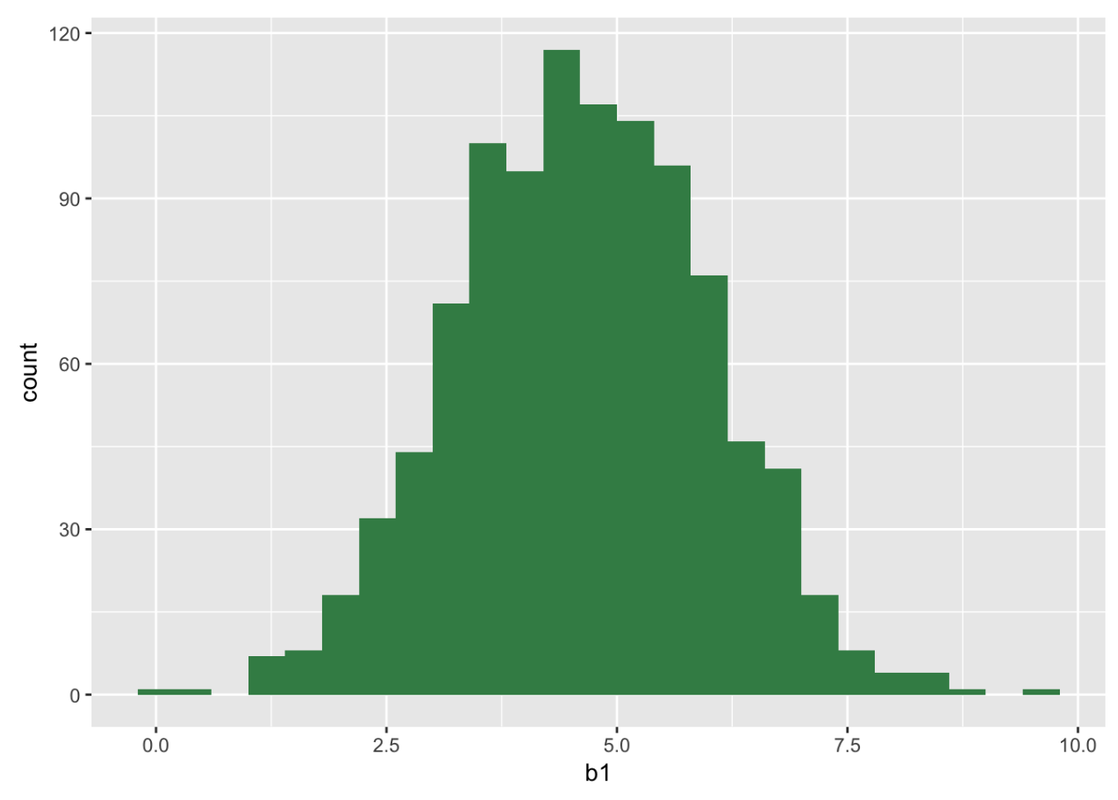
 -0.9966716 3.683187 4.579354 5.5494499 9.84942 4.640165 1.345508  1000       0

Note that the sampling distribution of the difference between two means (the estimate \(b_{1}\)) is normal in shape, just like the sampling distribution of means. The mean of the sampling distribution is close to 4.6, as it should be given that we are resampling from our sample observations, and the mean difference between Short and Tall in our sample was 4.6. The spread of this sampling distribution will give us an estimate of the standard error of the difference between the two groups.

Constructing the Confidence Interval of \(\beta_{1}\)

Having the created the bootstrapped sampling distribution of \(b_1\), let’s now use it to find the lower and upper bounds of the confidence interval.

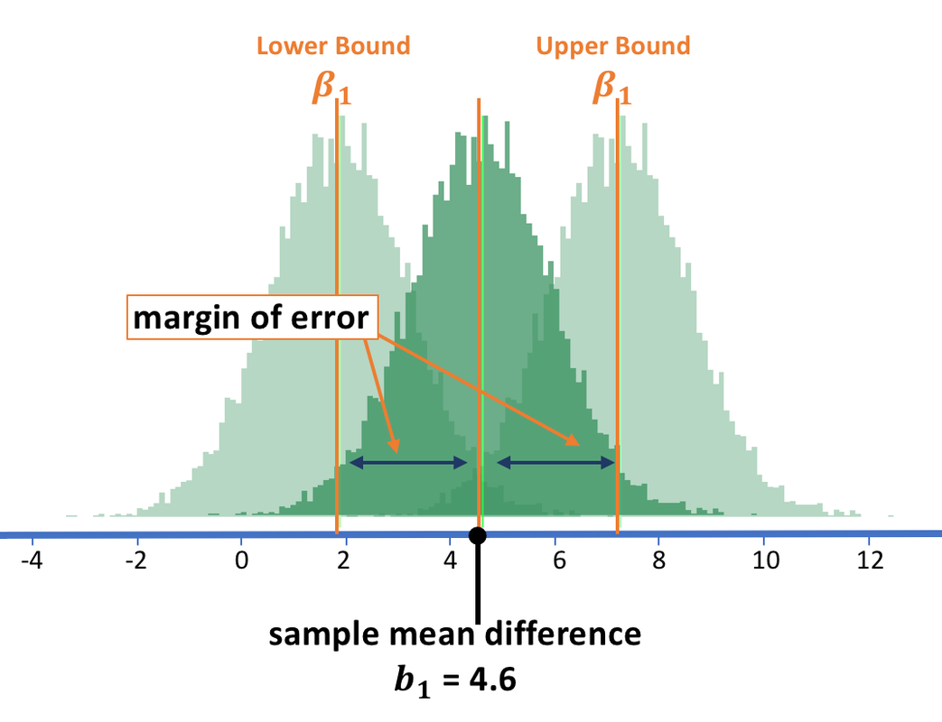
The light green sampling distribution centered at the lower bound \(\beta_1\) in the figure above shows you all the \(b_1\)s that could have been generated by that DGP. As you can see, the particular \(b_1\) in our study (4.6) would have less than a 2.5% change of being generated by a sampling distribution centered at the lower bound or lower. And the same reasoning applies for the upper bound.

Just as we did before, we can assume that the upper and lower bound \(\beta_1\)s will correspond to the upper and lower 2.5% cutoffs of the sampling distribution centered at our sample \(b_1\) of 4.6 (see graph above). The bootstrapped sampling distribution we created (dark green in the graph above) is indeed centered at 4.6, so we can use it to find the upper and lower bound cutoff points.

To find out where these cutoffs are, we can arrange our 1000 bootstrapped \(b_1\)s in order. The lower bound of the 95% confidence interval will be the point below which the lowest 25 \(b_1\)s are. The upper bound will be the point above which the 25 highest are.

In this code window, arrange b1 in bootSDob1 in order, and then print out the 25th and 975th values.

[1] 7.158011

[1] 2.061277

The 95% confidence interval for the true population difference in thumb lengths between Short and Tall people is between about 2 and 7.2 millimeters.

We can also find that the margin of error from each of these cutoffs to the mean of the bootstrapped sampling distribution is about 2.6. The margin of error represents how far above (and below) the upper bound \(\beta_1\) (and lower bound \(\beta_1\)) are from the estimate.

Interpreting the Confidence Interval of \(\beta_{1}\)

The bootstrapped confidence interval of \(\beta_1\) was 2 and 7.2 millimeters. We are quite confident in saying that \(\beta_1\) could perhaps be 2.1 or 3 or 6.8 or some other value between 2 and 7.2. Because 0 is not included in this 95% confidence interval, we are quite confident that the true difference between the two groups is not 0. After all, if the true difference is 0 then there is a less than 5% chance that we would have observed the sample mean that we observed. This being the case, we are probably going to want to maintain the more complex model (that is, the Height2Group model).

If 0 was included in our 95% confidence interval, we could consider it within the bounds of likely that there is no real difference in the population parameter between the Short group and the Tall group. This would have implications for which model we might prefer to represent the relationship between height and thumb length.

If, in the two-group model, \(\beta_1\) turned out to be 0, then we wouldn’t need the \(\beta_{1}X_{i}\) term in our model (0 times either 0 or 1 would still yield a 0). If \(\beta_1X_1\) were dropped out of the model, we would be left with the empty model, which is a simpler model:

\[Y_i=\beta_0+\epsilon_i\]

We would probably prefer the simpler model unless we were 95% certain that the group difference was real. If we were pretty confident (say, 95% confident) that \(\beta_{1}\) could not be 0, then we could reject the simple model in favor of the more complex one.

Using a Mathematical Model to Construct the Confidence Interval for \(\beta_{1}\)

As with the mean before, there is a way to shortcut all of this. Try the function confint() on Height2Group.model.

                     2.5 %    97.5 %
(Intercept)      55.941318 59.694251
Height2Grouptall  1.938845  7.263278

Notice that with a more complex model, we now get two sets of confidence intervals.

Because it is reasonable to assume that the sampling distribution of differences in means is approximately normal and well modeled by the t distribution, the confint() function uses it to find the cutoff points for the lower and upper 2.5% tails of the sampling distribution.

Now you can compare the 95% confidence intervals constructed using the two methods: bootstrapping and confint(). Bootstrapping estimated the confidence interval as between 2 and 7.2, which is pretty close to what we found from modeling the sampling distribution as a t distribution (1.9, 7.3).

Just like when we found the confidence interval through resampling, we would say that the complex model is different from the empty model, and we should make different predictions of thumb length for short and tall people.