Course Outline
-
segmentGetting Started (Don't Skip This Part)
-
segmentStatistics and Data Science: A Modeling Approach
-
segmentPART I: EXPLORING VARIATION
-
segmentChapter 1 - Welcome to Statistics: A Modeling Approach
-
segmentChapter 2 - Understanding Data
-
segmentChapter 3 - Examining Distributions
-
segmentChapter 4 - Explaining Variation
-
segmentPART II: MODELING VARIATION
-
segmentChapter 5 - A Simple Model
-
segmentChapter 6 - Quantifying Error
-
segmentChapter 7 - Adding an Explanatory Variable to the Model
-
segmentChapter 8 - Models with a Quantitative Explanatory Variable
-
8.3 Using the Regression Model to Make Predictions
-
segmentPART III: EVALUATING MODELS
-
segmentChapter 9 - Distributions of Estimates
-
segmentChapter 10 - Confidence Intervals and Their Uses
-
segmentChapter 11 - Model Comparison with the F Ratio
-
segmentChapter 12 - What You Have Learned
-
segmentFinishing Up (Don't Skip This Part!)
-
segmentResources
list full book
8.3 Using the Regression Model to Make Predictions
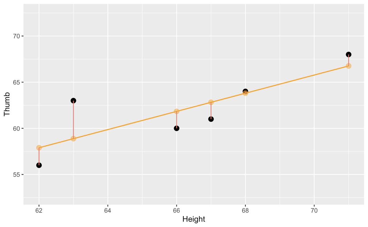
The specific regression line, defined by its slope and intercept, is the one that fits our data best. By this we mean that this model reduced leftover error to the smallest level possible given our variables. Specifically, the sum of squared deviations around this line are the lowest of any possible line we could have used instead.
Like the empty and group models, error around the regression line is also balanced. You can almost imagine the data points each pulling on the regression line and the best fitting regression line balances the “pulls” above and below it.
This regression model also is our best estimate of the relationship between height and thumb length in the population. As with other models of the population, we can use the regression model to predict future observations. To do so we must turn it into a function, one that will predict thumb length based on height.
Here is the fitted model for using Height to predict Thumb based on the complete Fingers data set:
\[Thumb_{i}= -3.33+.96*Height_{i}+e_{i}\]
Remember, a function takes in some input and spits out a prediction based on a model. Here is the function we can use to predict a thumb length based on a person’s height:
predicted Thumb \(=-3.33+.96*Height_{i}\)
We can write this more generally by replacing the variable Thumb with \(Y_i\) and the variable Height with \(X_i\). And since \(Y_i\) actually represents the collected data for Thumb, we put a little hat over the Y, like this \(\hat{Y}\), to indicate that these are the predicted thumb lengths.
\[\hat{Y}=-3.33+.96*X_{i}\]
With the two-group model it was easy to make predictions from the model: no calculation was required to see that if the person was short, the prediction would be the mean for short people; and if the person was tall, the prediction would be the mean for tall people. But with the regression model it’s harder to do the calculation in your head.
Remember the b0() and b1() functions we used on page 7.3? We can use them to pull out the parameter estimates from our best fitting model. For example, this code will return the \(b_0\) from our model.
b0(Height.model)If we wanted to generate a predicted thumb length using the Height.model for someone who is 60 inches tall, we could write:
b0(Height.model) + b1(Height.model)*60Using the window below, and the b0() and b1() functions, see if you can write a line of R code that would return the predicted thumb length for someone who is 73.5 inches tall based on the parameter estimates of the Height.model.
            require(tidyverse)
            require(mosaic)
            require(Lock5Data)
            require(supernova)

            Fingers <- filter(Fingers, Thumb >= 33 & Thumb <= 100)
            # this creates the best fitting Height.model
            Height.model <- lm(Thumb ~ Height, data = Fingers)

            # What would the Height.model predict for the Thumb length
            # of someone who is 73.5 inches tall?
            # this creates the best fitting Height.model
            Height.model <- lm(Thumb ~ Height, data = Fingers)

            # What would the Height.model predict for the Thumb length
            # of someone who is 73.5 inches tall?
            b0(Height.model) + b1(Height.model) * 73.5
            ex() %>% check_or(
                check_operator(., "+") %>% check_result() %>% check_equal(),
                check_output_expr(., b0(Height.model) + b1(Height.model) * 73.5),
                check_output(., "67.36895"),
                check_output(., "67.369"),
                check_output(., "67.37"),
                check_output(., "67.4")
            )
[1] 67.36895This code works fine for making individual predictions, but to check our model against the data, we would want to generate predictions for each student in the Fingers data frame. As we’ve said before, we really don’t need predictions when we already know their actual thumb lengths. But this is a way to see how well (or how poorly) the model would have predicted the thumb lengths for the students in our data set.
We will use the predict() function, which you have used before, to make a new variable with the predictions based on Height.model. We’ll save those predictions as Height.pred.
Fingers$Height.pred <- predict(Height.model)Then we’ll print out the first 10 rows of the data frame—but only the variables Thumb length, Height, and the predicted thumb length from the Height model.
head(select(Fingers, Thumb, Height, Height.pred), 10) Thumb Height Height.pred
1 66.00 70.5 64.48330
2 64.00 64.8 59.00056
3 56.00 64.0 58.23105
4 58.42 70.0 64.00235
5 74.00 68.0 62.07859
6 60.00 68.0 62.07859
7 70.00 69.0 63.04047
8 55.00 65.7 59.86625
9 60.00 62.5 56.78823
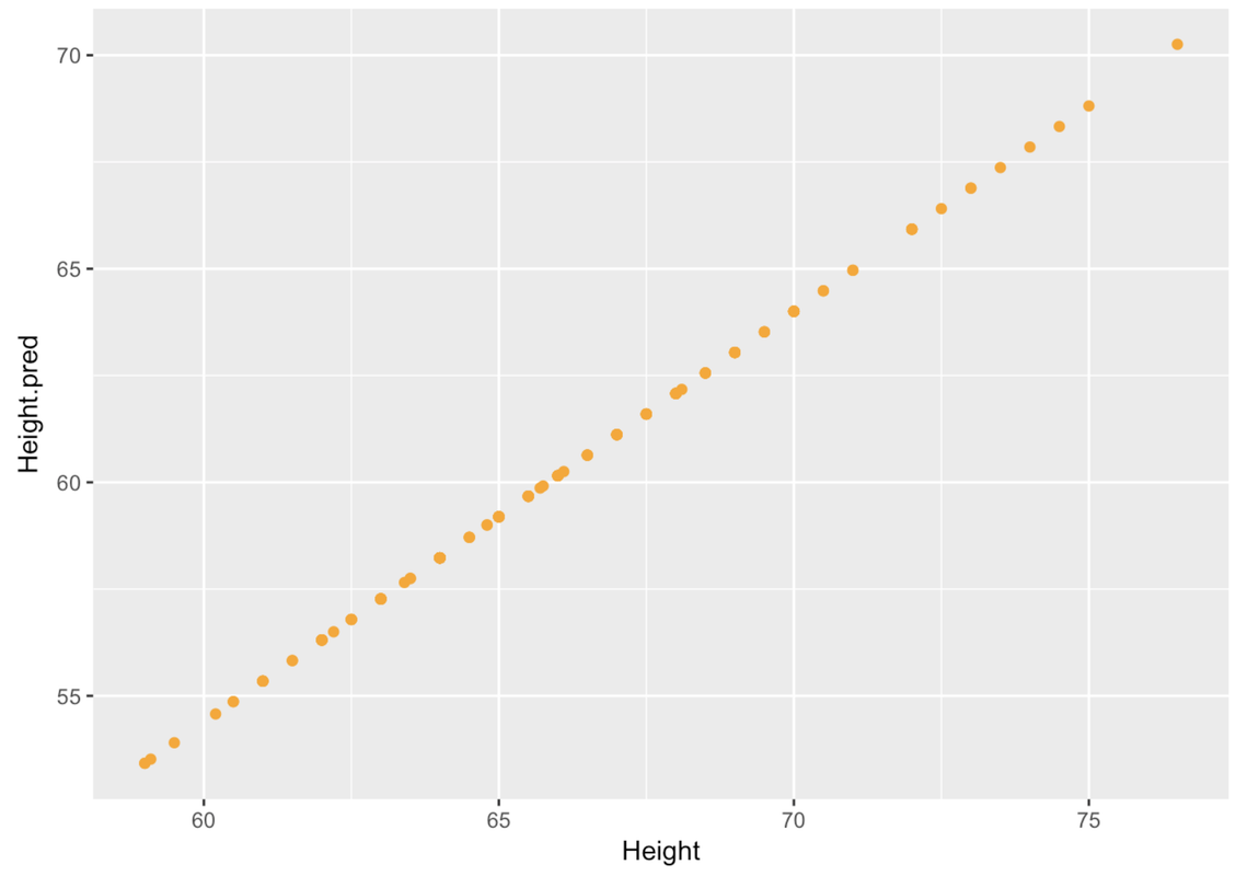
10 52.00 63.4 57.65392We’ve added the code to calculate Height.pred in the code window below. Add the code to create the scatter plot of Height.pred (y-axis) by Height (x-axis) using gf_point in the code window below.
            require(tidyverse)
            require(mosaic)
            require(Lock5Data)
            require(supernova)

            Fingers <- filter(Fingers, Thumb >= 33 & Thumb <= 100)
            Height.model <- lm(Thumb ~ Height, data = Fingers)
            # this creates predicted thumb lengths from Height.model
            Fingers$Height.pred <- predict(Height.model)

            # write code to create a scatter plot of Height.pred by Height
            gf_point()
            # this creates predicted thumb lengths from Height.model
            Fingers$Height.pred <- predict(Height.model)

            # write code to create a scatter plot of Height.pred by Height
            gf_point(Height.pred ~ Height, data = Fingers)
ex() %>% check_function("gf_point") %>% check_result() %>% check_equal()