9.4 The P-Value
Locating the Sample \(b_1\) in the Sampling Distribution
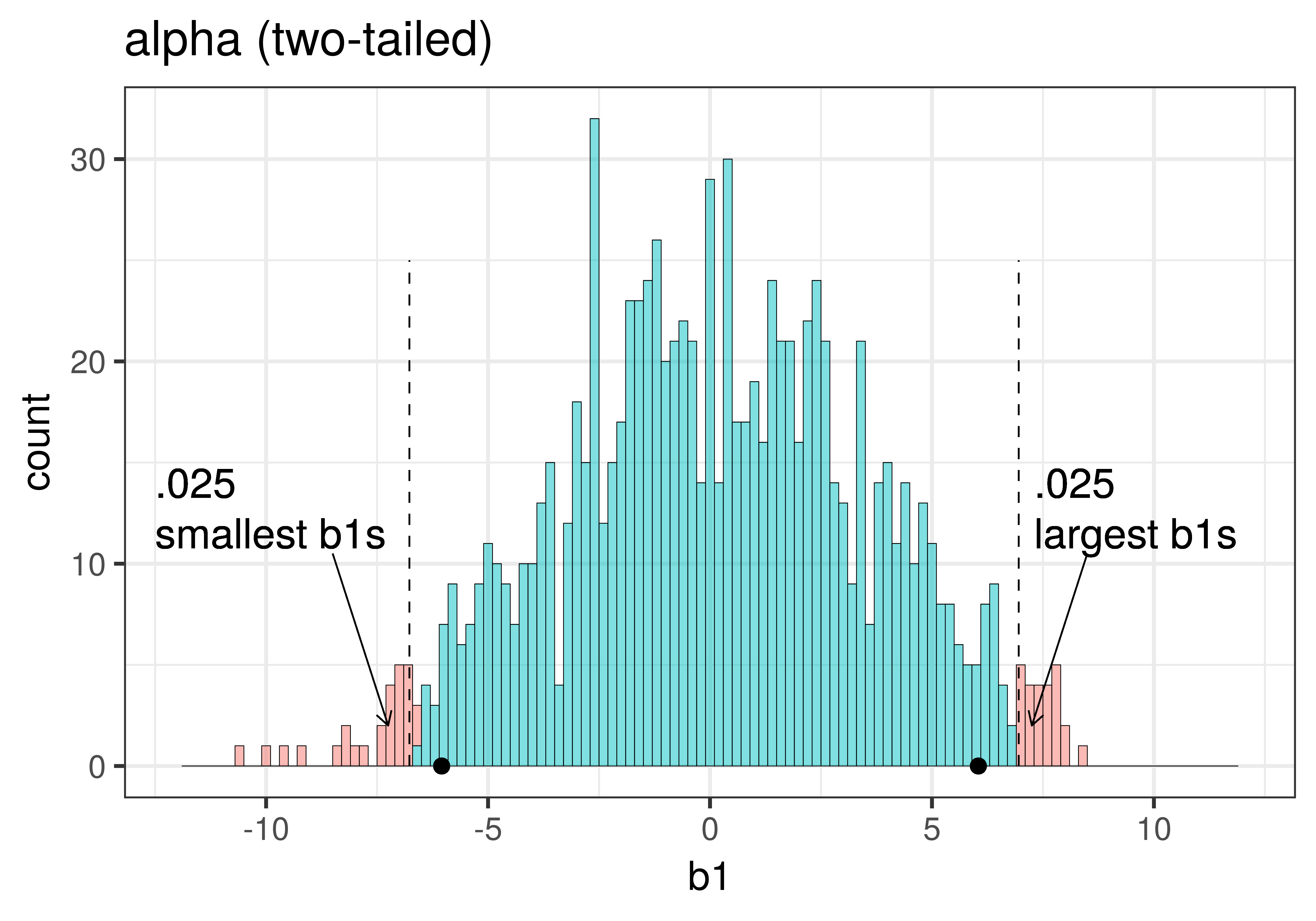
We have now spent some time looking at the sampling distribution of \(b_1\)s assuming the empty model is true (i.e., \(\beta_1=0\)). We have developed the idea that simulated samples, generated by random shuffles of the tipping experiment data, are typically clustered around 0. Samples that end up in the tails of the distribution – the upper and lower .025 of values – are considered unlikely.
Let’s place our sample \(b_1\) right onto our histogram of the sampling distribution and see where it falls. Does it fall in the tails of the distribution, or in the middle .95?
Here’s some code that will save the value of our sample \(b_1\) as sample_b1.
sample_b1 <- b1(Tip ~ Condition, data = TipExperiment)If we printed it out, we would see that the sample \(b_1\) is 6.05: tables in the smiley face condition, on average, tipped $6.05 more than tables in the control condition.
Let’s find out by overlaying the sample \(b_1\) onto our histogram of the sampling distribution. Chaining the code below onto the histogram above (using the %>% operator) will place a black dot right at the sample \(b_1\) of 6.05:
gf_point(x = 6.05, y = 0)If you have already saved the value of \(b_1\) (as we did before, into sample_b1), you can also write the code like this:
gf_point(x = sample_b1, y = 0)
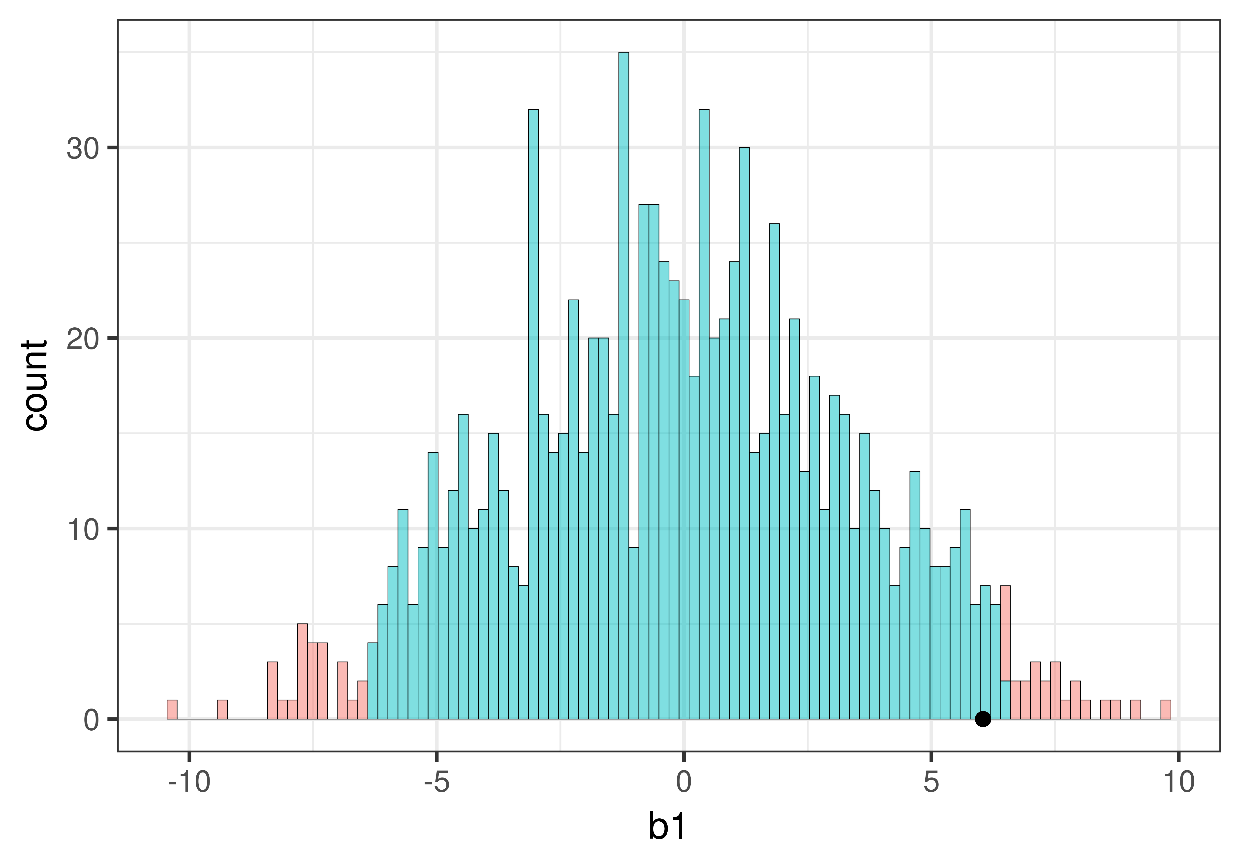
We can see that our sample is not in the unlikely zone. It’s within the middle .95 of \(b_1\)s generated from the empty model of the DGP.
Recap of Logic with the Distribution Triad
The hard thing about inference is that we have to keep all three distributions (sample, DGP, and sampling distribution) in mind. It’s really easy to lose track. We’re going to introduce a new kind of picture that shows all three of these distributions together in relation to one another.
The picture below represents how we’ve used sampling distributions so far to evaluate the empty model (or null hypothesis). Let’s start from the top of this image. The top blue horizontal line represents the possible values of \(\beta_1\) in the DGP. The true value of \(\beta_1\) is unknown; it’s what we are trying to find out. But we’ve hypothesized that it might be 0, so we have represented that in the red box.
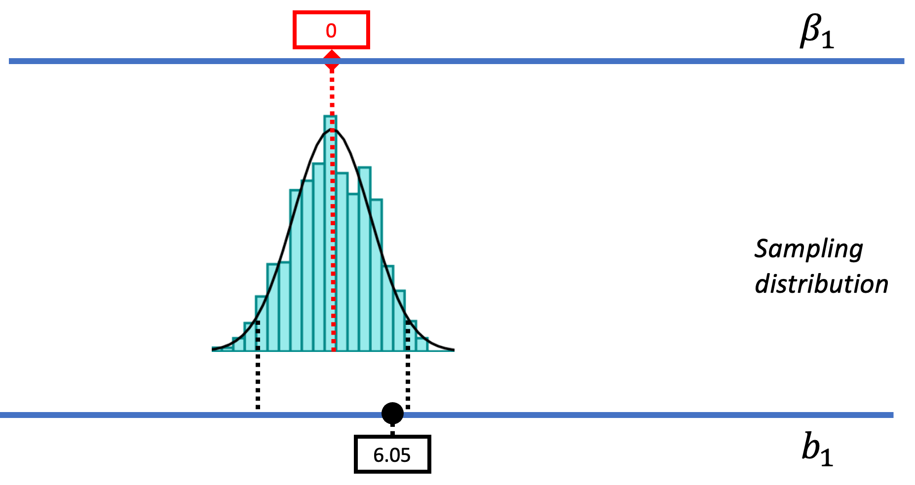
Based on this hypothesized DGP, we simulated samples, generated by random shuffles of the tipping experiment data. These sample \(b_1\)s tend to be clustered around 0 because we were simulating the empty model in which \(\beta_1=0\). Samples that end up in the tails of the distribution – the upper and lower .025 of values – are considered unlikely. We have drawn in black dotted lines to represent the cutoffs, the boundaries separating the middle values (not considered unlikely) from the values in the upper and lower tails (considered unlikely).
The Concept of P-Value
We have located the sample \(b_1\) in the context of the sampling distribution generated from the empty model, and we have seen that it falls in the middle .95 of \(b_1\)s. If it had fallen in either of the two tails, we would judge it unlikely to have been generated by the empty model, which might lead us to reject the empty model.
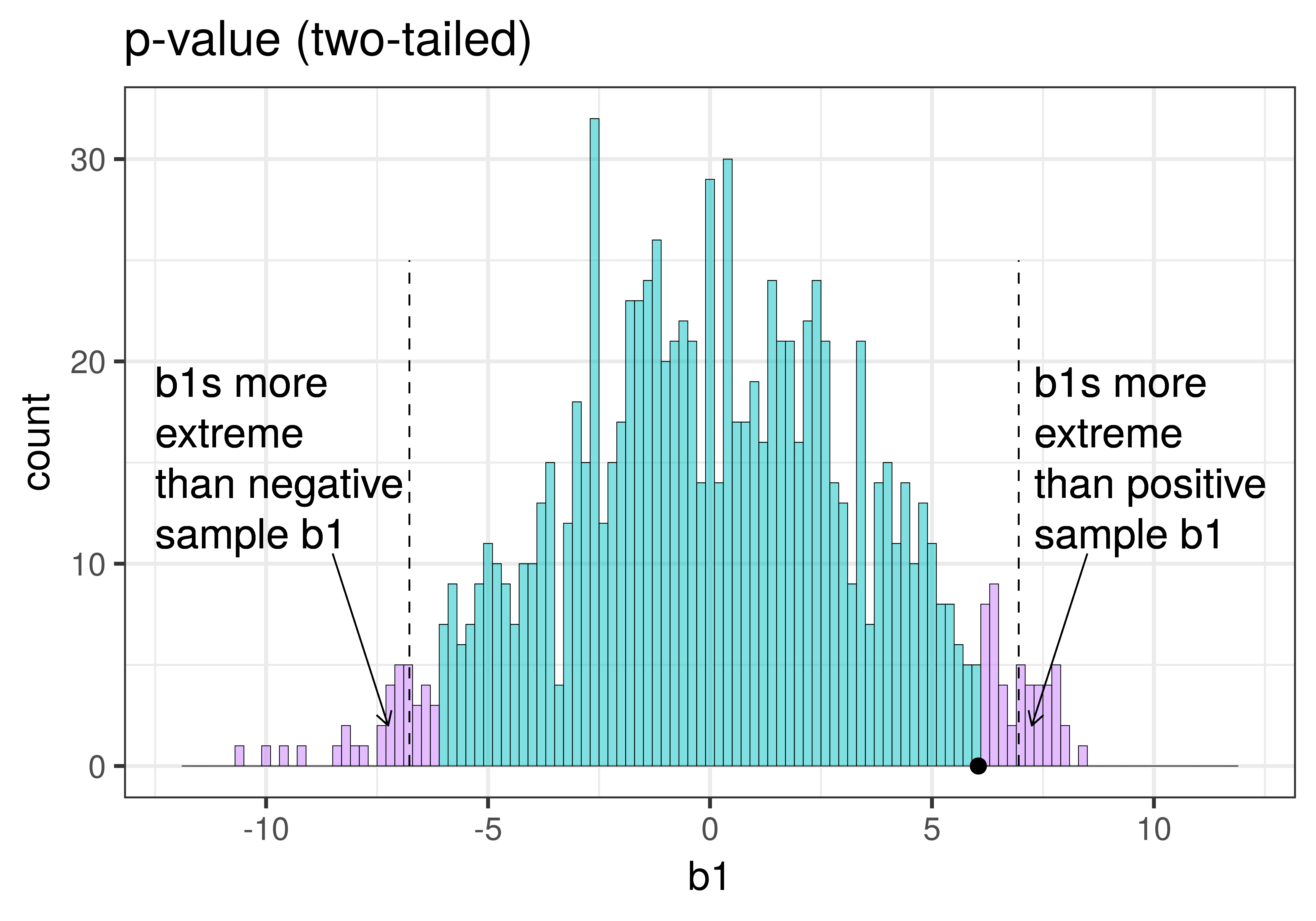
But we can do better than this. We don’t have to just ask a yes/no question of our sampling distribution. Instead of asking whether the sample \(b_1\) is in the unlikely area or not (yes or no), we could instead ask, what is the probability of getting a \(b_1\) as extreme as the one observed in the actual experiment? The answer to this question is called the p-value.
Before we teach you how to calculate a p-value, let’s do some thinking about what the concept means.
The total area of the two tails shaded red in the histogram above represent the alpha level of .05. These regions represent the \(b_1\)s generated from the empty model that we have decided to judge as unlikely based on our alpha. This means that if the empty model is true, as we assumed when we constructed the sampling distribution, then the probability of getting a sample \(b_1\) in the red region would be .05.
Whereas we know what alpha is before we even do a study – it’s just a statement of our criterion for deciding what we will count as unlikely – the p-value is calculated after we do a study, based on actual sample data. We can illustrate the difference between these two ideas in the plots below, which zero in on just the upper tail of the sampling distribution of \(b_1\).
| alpha | p-value |
|---|---|
| This plot illustrates the concept of alpha. Having decided to set alpha as .05, the red area in the upper tail of the sampling distribution represents .025 of the largest \(b_1\)s generated by the empty model. | This plot illustrates the concept of p-value. While p-value is also a probability, it is not dependent on alpha. P-value is represented by the purple area beyond our sample \(b_1\) and is the probability of getting a \(b_1\) greater than our sample \(b_1\). |
|
|
|
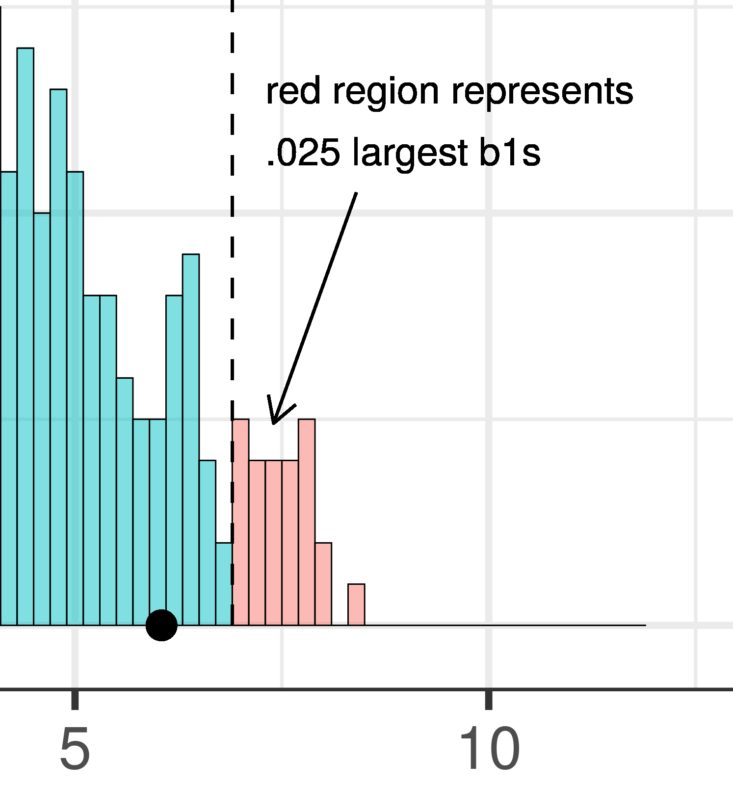
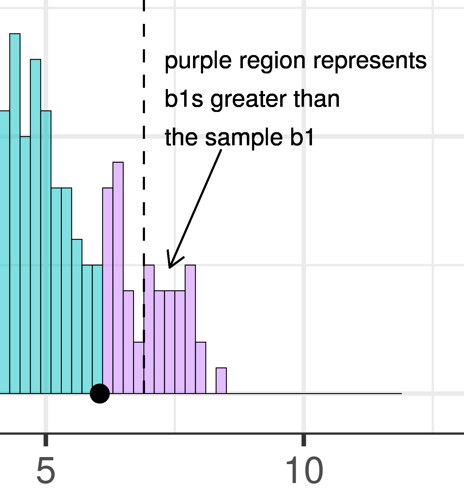
The dashed line in the plot on the left has been added to demarcate the cutoff beyond which we will consider unlikely, and the middle .95 of the sampling distribution which we consider not unlikely. We have kept the dashed line in the plot on the right to help you remember where the red alpha region started.
In the pictures above, we showed only the upper tail of the sampling distribution. But because a very low \(b_1\) (for example, -9) would also make us doubt the empty model of the DGP, we will want to do a two-tailed test. In the plots below we have zoomed out to show both tails of the sampling distribution, again illustrating alpha (with the red tails) and p-value (with the purple tails).
|
|---|
|
Because the purple tails, which represent the area beyond the sample \(b_1\), are a bit larger than the red tails, which represent the alpha of .05, we would guess that the p-value is a bit bigger than .05. But it’s not that much bigger – certainly not as large as .40 or .80!
The p-value is the probability of getting a parameter estimate as extreme or more extreme than the sample estimate given the assumption that the empty model is true.
Thus, the p-value is calculated based on both the value of the sample estimate and the shape of the sampling distribution of the parameter estimate under the empty model. In contrast, alpha does not depend on the value of the sample estimate.
Calculating the P-Value for a Sample
To calculate the probability of getting a \(b_1\) within a particular region (e.g., greater than $6.05 and less than -$6.05) we can simply calculate the proportion of \(b_1\)s in the sampling distribution that fall within these regions. In this way, we are using the simulated sampling distribution of 1000 \(b_1\)s as a probability distribution.
We can use tally() to figure out how many simulated samples are more extreme than our sample \(b_1\). The first line of code will tell us how many \(b_1\)s are more extreme on the positive side than our sample_b1 ($6.05), the second line, how many are more extreme than our sample on the negative side (-$6.05).
tally(~ b1 > sample_b1, data = sdob1)
tally(~ b1 < -sample_b1, data = sdob1)
(Coding note: R thinks of <- with no space between the two characters as an assignment operator; it’s supposed to look like an arrow. For the second line of code, you need to be sure to put a space between the < and - so R interprets it to mean less than the negative of sample_b1.)
The two lines of tally() code will produce:
b1 > sample_b1
 TRUE FALSE
   38   963
b1 < -sample_b1
 TRUE FALSE
   41   959
When we add up the two tails (the extreme positive \(b_1\)s and negative \(b_1\)s), there are about 80 \(b_1\)s that are more extreme than our sample \(b_1\).
Since there are about 80 randomly generated \(b_1\)s (out of a 1000) that are more extreme than our sample, we would say there is roughly a .08 likelihood of the empty model generating a sample as extreme as $6.05. This probability is the p-value.
tally(~ b1 > sample_b1, data = sdob1)
tally(~ b1 < -sample_b1, data = sdob1)
Instead of using two lines of code - one to find the number of \(b_1\)s at the upper extreme, the other at the lower extreme - we can use a single line of code like this:
tally(sdob1$b1 > sample_b1 | sdob1$b1 < -sample_b1)Note the use of the | operator, which means or, to put the two criteria together: this code tallies up the total number of \(b_1\)s that are either greater than positive $6.05 or less than negative $6.05. You can run the code in the code window below. Try adding the argument format = "proportion" to get the proportion or p-value directly.
require(coursekata)
# this saves the sample b1 and creates a sampling distribution using shuffle
            sample_b1 <- b1(Tip ~ Condition, data = TipExperiment)
            sdob1 <- do(1000) * b1(shuffle(Tip) ~ Condition, data = TipExperiment)

            # change the code below to calculate the *proportion* of b1s
            # as extreme (positive or negative) as the sample b1
            tally(sdob1$b1 > sample_b1 | sdob1$b1 < -sample_b1)
# this saves the sample b1 and creates a sampling distribution using shuffle
         sample_b1 <- b1(Tip ~ Condition, data = TipExperiment)
            sdob1 <- do(1000) * b1(shuffle(Tip) ~ Condition, data = TipExperiment)

         # change the code below to calculate the *proportion* of b1s
            # as extreme (positive or negative) as the sample b1
         tally(sdob1$b1 > sample_b1 | sdob1$b1 < -sample_b1, format="proportion")
ex() %>%
    check_function("tally") %>% {
       check_arg(., "format") %>% check_equal()
       check_result(.) %>% check_equal()
}The p-value for the \(b_1\) in the tipping experiment was .08, which is greater than our alpha of .05. Therefore, we would say our sample is not unlikely to have been generated by this DGP. Thus, we would consider the empty model a plausible model of the DGP and therefore not reject the empty model. Even a DGP where there is no effect of smiley face can produce a \(b_1\) that is as extreme as our sample or more extreme about .08 of the time.
If our p-value had been less than .05, we might have declared our sample unlikely to have been generated by the empty model of the DGP, and thus rejected the empty model.
What It Means to Reject – or Not – the Empty Model (or Null Hypothesis)
The concept of p-value, and using it to decide whether or not to reject the empty model in favor of the more complex model we have fit to the data, comes from a tradition known as Null Hypothesis Significance Testing (NHST). The null hypothesis is, in fact, the same as what we call the empty model. It refers to a world in which \(\beta_1=0\).
While we want you to understand the logic of NHST, we also want you to be thoughtful in your interpretation of the p-value. The NHST tradition has been criticized lately because it often is applied thoughtlessly, in a highly ritualized manner (download NHST article by Gigerenzer, Krauss, & Vitouch, 2004 (PDF, 286KB)). People who don’t really understand what the p-value means may draw erroneous conclusions.
For example, we just decided, based on a p-value of .08, to not reject the empty model of Tip. But does this mean that \(\beta_1\) in the true DGP is actually equal to 0? No. This means it could be 0, and the data are consistent with it being 0. But it could be something else instead.
It could, for example, be 6.05, which was the best-fitting estimate of \(\beta_1\) based on the sample data. If the true \(\beta_1\) were equal to 6.05, we could be sure that 6.05 would be one of the many possible \(b_1\)s that would be considered likely.
If both the empty model and the complex “best-fitting” model are possible true models of the DGP, how should we decide which model to use?
Some people from the null hypothesis testing tradition would say that if you cannot reject the empty model then you should use the empty model. From this perspective, we should avoid Type I error at all costs; we don’t want to say there is an effect of smiley face when there is not one in the DGP. In this tradition, it is worse to make a Type I error than a Type II error, to say there is no effect when there is, in fact, an effect in the DGP.
But this might not be the best course of action in some situations. For example, if you simply want to make better predictions, you might decide to use the complex model, even if you cannot rule out the empty model. On the other hand, if your goal is to better understand the DGP, there is some value in having the simplest theory that is consistent with your data. Scientists call this preference for simplicity “parsimony.”
Judd, McClelland, and Ryan (some statisticians we greatly admire) once said that you just have to decide whether a model is “better enough to adopt.” Much of statistical inference involves imagining a variety of models that are consistent with your data and looking to see which ones will help you to achieve your purpose.
We prefer to think in terms of model comparison instead of null hypothesis testing. With too much emphasis on null hypothesis testing, you might think your job is done when you either reject or fail to reject the empty model. But in the modeling tradition, we are always seeking a better model: one that helps us understand the DGP, or one that makes better predictions about future events.