13.5 Using shuffle() for Targeted Model Comparisons (Part 1)
Using the shuffle() function to generate sampling distributions for targeted model comparisons is a little more complicated than for the overall model. As an example, let’s see how we could use shuffle() to generate a sampling distribution to help us interpret HomeSizeK F in the multivariate model. Again, these are the two models we are comparing:
| Model | GLM Notation |
|---|---|
| Complex | \(PriceK_i = \beta_0 + \beta_1NeighborhoodEastside_i + \beta_2HomeSizeK_i + \epsilon_i\) |
| Simple | \(PriceK_i= \beta_0 + \beta_1NeighborhoodEastside_{i} + \colorbox{yellow}{(0)}HomeSizeK_{i} + \epsilon_i\) |
Our question is: what is the probability (the p-value) that the additional variability in PriceK explained by HomeSizeK over and above that explained by Neighborhood could simply be due to random sampling variation? In other words, could the F for HomeSizeK have resulted from the simple model of the DGP?
Let’s first recall how we used shuffle() to mimic the DGP for the empty model:
shuffle(PriceK) ~ Neighborhood + HomeSizeK
This code effectively broke the relationship between both of the predictor variables and PriceK. When we shuffle PriceK we are shuffling not only the part related to home size, but also the part related to neighborhood. Is there a way to first take out the effect of Neighborhood and look only at the parts of PriceK that might be predicted by HomeSizeK?
We actually have learned a way to isolate just the part of PriceK that is related to Neighborhood, and that is to fit the neighborhood model and save the leftover variation (i.e., residuals).
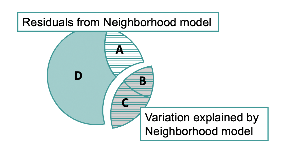
These residuals (region A+D in the Venn diagram above) represent just the part of PriceK that might be uniquely predicted by HomeSizeK. If we shuffle them, we are mimicking the simple model in which HomeSizeK has no effect beyond that accounted for by Neighborhood.
| Model | R Code | GLM Notation |
|---|---|---|
| Simple |
shuffle(residuals) ~ Neighborhood + HomeSizeK
|
\(PriceK_i= \beta_0 + \beta_1NeighborhoodEastside_{i} + \colorbox{yellow}{(0)}HomeSizeK_{i} + \epsilon_i\) |
The two-step method experts recommend for using shuffle() to create a sampling distribution to test just the effect of HomeSizeK is based on this idea. Step one is to fit the Neighborhood model of PriceK and save the residuals. Step two is to shuffle these residuals and use them as the outcome variable in a regression with both Neighborhood and HomeSizeK as predictors.
If we shuffle this new outcome variable (the residuals) we will be mimicking a DGP in which HomeSizeK has no effect on the leftover variation, but still maintains the relationship between the two predictors (HomeSizeK and Neighborhood).
If we fit a regression model to the the shuffled residuals many times and record the F for HomeSizeK for each iteration we will get a sampling distribution assuming a DGP in which HomeSizeK has no effect over and above that already accounted for by Neighborhood. The sample F we will use for comparison is the one on the HomeSizeK row of the supernova table for the multivariate model.
Let’s go through this process one step at a time, and spend some time thinking about the results at each step of the way.
Step One: Save Residuals from the Neighborhood Model
In the code window below we’ve put in some code to fit the neighborhood model of price (PriceK ~ Neighborhood). Write some code to save the residuals from the Neighborhood_model as PriceK_N_resid).
require(coursekata)

# delete when coursekata-r updated
Smallville <- read.csv("https://docs.google.com/spreadsheets/d/e/2PACX-1vTUey0jLO87REoQRRGJeG43iN1lkds_lmcnke1fuvS7BTb62jLucJ4WeIt7RW4mfRpk8n5iYvNmgf5l/pub?gid=1024959265&single=true&output=csv")
Smallville$Neighborhood <- factor(Smallville$Neighborhood)
Smallville$HasFireplace <- factor(Smallville$HasFireplace)
# this fits and saves the neighborhood model
Neighborhood_model <- lm(PriceK~ Neighborhood, data = Smallville)

# write code to  save the residuals of the neighborhood model
PriceK_N_resid <-

# this will print a few of these residuals
head(PriceK_N_resid)
Neighborhood_model <- lm(PriceK~ Neighborhood, data = Smallville)
PriceK_N_resid <- resid(Neighborhood_model)
head(PriceK_N_resid)
# temporary SCT
ex() %>% check_error()Is the Effect of Home Size Still There in the Residuals?
Now that we have saved the residuals from the single-predictor neighborhood model, we can fit the multivariate model using residuals from the neighborhood model as the outcome variable (PriceK_N_resid = Neighborhood + HomeSizeK) to make sure the effect of HomeSizeK is unchanged.
require(coursekata)

# delete when coursekata-r updated
Smallville <- read.csv("https://docs.google.com/spreadsheets/d/e/2PACX-1vTUey0jLO87REoQRRGJeG43iN1lkds_lmcnke1fuvS7BTb62jLucJ4WeIt7RW4mfRpk8n5iYvNmgf5l/pub?gid=1024959265&single=true&output=csv")
Smallville$Neighborhood <- factor(Smallville$Neighborhood)
Smallville$HasFireplace <- factor(Smallville$HasFireplace)

# this fits and saves the neighborhood model
Neighborhood_model <- lm(PriceK~ Neighborhood, data = Smallville)
# this saves the residuals of the neighborhood model
PriceK_N_resid <- resid(Neighborhood_model)

# write code to fit the multivariate model again, this time
# using residuals from the neighborhood model as the outcome variable
PriceK_N_resid_multi_model <- lm()

# this will print the ANOVA table for this new model
supernova(PriceK_N_resid_multi_model)
PriceK_N_resid <- resid(Neighborhood_model)
PriceK_N_resid_multi_model <- lm(PriceK_N_resids ~ Neighborhood + HomeSizeK, data = Smallville)
supernova(PriceK_N_resid_multi_model)
# temporary SCT
ex() %>% check_error()We have printed out two ANOVA tables below. The first is the one we just got by fitting the multivariate model to the residuals of the neighborhood model (PriceK_N_resids), the second, the original multivariate model with PriceK as the outcome variable.
It is useful to compare these two tables and try to understand their similarities and differences. Notice that the model of residuals has a much smaller SS Total than the original model of PriceK.
Analysis of Variance Table (Type III SS)
Model: PriceK_N_resid ~ Neighborhood + HomeSizeK

                                        SS df        MS      F    PRE     p
 ------------ --------------- | ---------- -- --------- ------ ------ -----
        Model (error reduced) |  42003.677  2 21001.838  5.813 0.2862 .0075
 Neighborhood                 |   8237.712  1  8237.712  2.280 0.0729 .1419
    HomeSizeK                 |  42003.677  1 42003.677 11.626 0.2862 .0019
        Error (from model)    | 104774.465 29  3612.913
 ------------ --------------- | ---------- -- --------- ------ ------ -----
        Total (empty model)   | 146778.142 31  4734.779
Analysis of Variance Table (Type III SS)
Model: PriceK ~ Neighborhood + HomeSizeK

                                       SS df        MS      F    PRE     p
 ------------ --------------- | ---------- -- --------- ------ ------ -----
        Model (error reduced) | 124403.028  2 62201.514 17.216 0.5428 .0000
 Neighborhood                 |  27758.259  1 27758.259  7.683 0.2094 .0096
    HomeSizeK                 |  42003.677  1 42003.677 11.626 0.2862 .0019
        Error (from model)    | 104774.465 29  3612.913
 ------------ --------------- | ---------- -- --------- ------ ------ -----
        Total (empty model)   | 229177.493 31  7392.822
The important thing to notice about these two ANOVA tables is that the rows for HomeSizeK and SS Error are identical. We now have a model that perfectly calculates the size of the HomeSizeK effect while controlling for neighborhood. The effect of home size (SS, F, PRE) is identical in the two tables. Notice that the F for the unique effect of HomeSizeK is 11.626.
Now, because the neighborhood effect has already been taken out, we can shuffle the residuals to break only the unique connection of home size to the outcome. By doing this repeatedly, we can create a sampling distribution of F for HomeSizeK that assumes no effect of home size, yet still controls for neighborhood.