10.5 Using F to Test a Regression Model
We can use sampling distributions of \(b_1\) or \(F\) to compare the empty model versus a two-group model. It turns out we can do the same for regression models. In chapter 9, we used a sampling distribution of \(b_1\) to test the \(b_1\) in a regression model. Now let’s use the F-distribution to see how the F ratio from a regression model compares to the Fs generated by the empty model of the DGP.
Recap: Using Check to Predict Tips
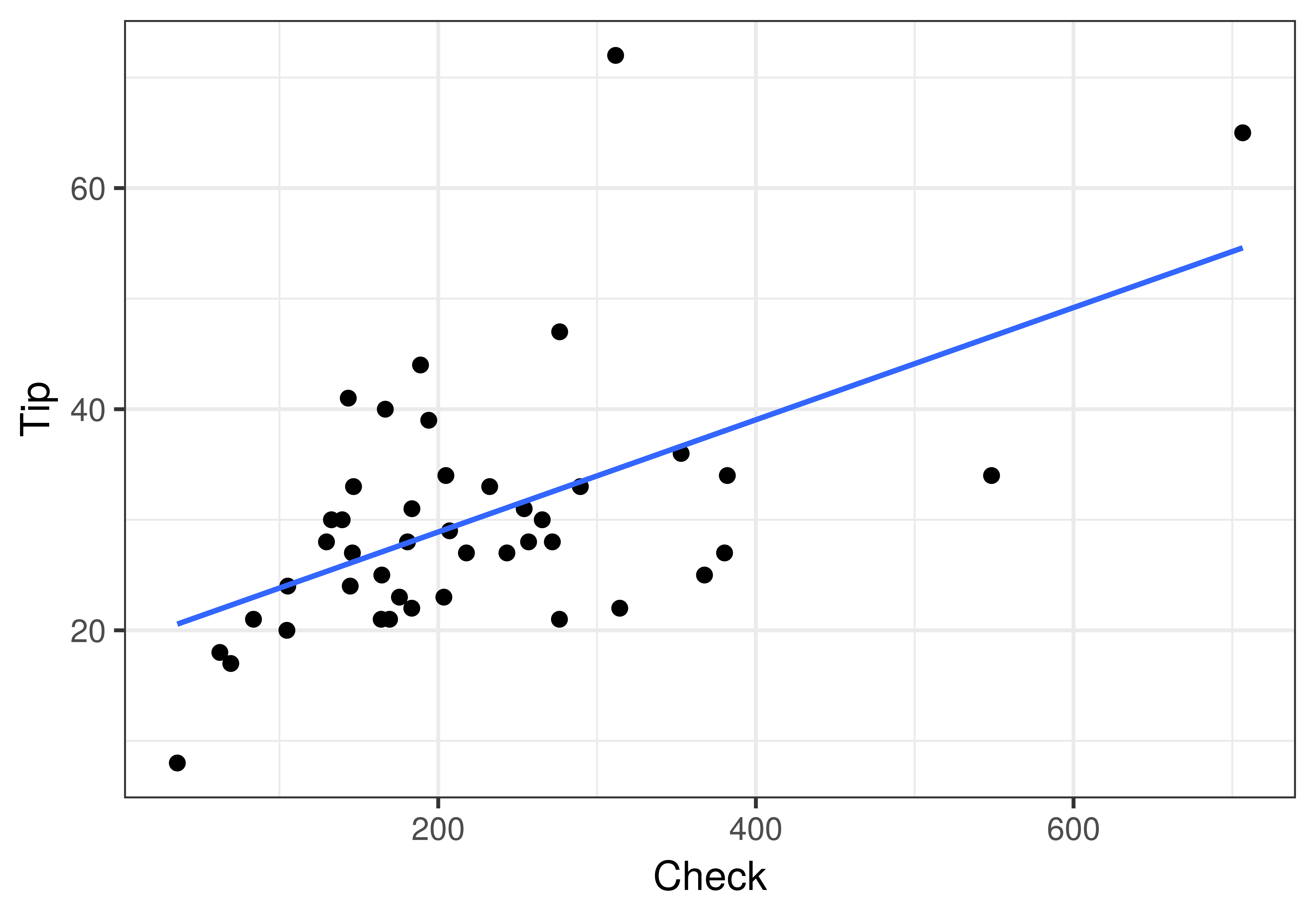
In Chapter 9 we created a regression model that used the total check for each table (Check) to predict the outcome Tip. We were interested in exploring the model: Tip = Check + Other Stuff. To remind us of this example, here is a scatterplot of the data as well as the best fitting regression model depicted as a blue line.
gf_point(Tip ~ Check, data = TipExperiment) %>%
gf_lm(color = "blue")
Using lm(), we fit the regression model and found the best fitting parameter estimates:
lm(Tip ~ Check, data = TipExperiment)Call:
lm(formula = Tip ~ Check, data = TipExperiment)
Coefficients:
(Intercept) Check
18.74805 0.05074The best-fitting \(b_1\) estimate was 0.05, meaning that for every one dollar increase in the total check, the Tip increased, on average, by 5 cents. This is the slope of the regression line. But while this is the best-fitting estimate of the slope based on the data, is it possible that this \(b_1\) could have been generated by the empty model, one in which the true slope in the DGP is 0?
In Chapter 9 we asked this question using the sampling distribution of \(b_1\). But we can ask the same question using the sampling distribution of F. Let’s start by finding the F for the Check model. You can do this in the code window below using the fVal() function.
require(coursekata)

# Simulate Check
set.seed(22)
x <- round(rnorm(1000, mean=15, sd=10), digits=1)
y <- x[x > 5 & x < 30]
TipPct <- sample(y, 44)
TipExperiment$Check <- (TipExperiment$Tip / TipPct) * 100
# calculate the sample F for the Check model
fVal()
# calculate the sample F for the Check model
fVal(Tip ~ Check, data = TipExperiment)
ex() %>% {
       check_function(., "fVal") %>%
       check_result() %>%
       check_equal()
}18.8653561562528The F ratio for the Check model is 18.87, which suggests that the variance explained by the model is 18.87 times the variance left unexplained by the model. Clearly, the Check model explains more variation than the empty model in the data.
But is it possible that the sample F could have been generated by a DGP in which there is no effect of Check on Tip? To answer this question we will need the sampling distribution of F generated under the empty model in which the true slope of the regression line in the DGP is 0.
Creating a Sampling Distribution of F
Following the same approach as we used for group models, we can use shuffle() to simulate many samples from a DGP in which there is no effect of Check on Tip, fit the Check model to each shuffled sample, and then calculate the corresponding value of F.
Write code to create a randomized sampling distribution of 1000 Fs (called sdoF) under the assumption that Check has no relationship with Tip. Print the first six lines of sdoF.
require(coursekata)

# Simulate Check
set.seed(22)
x <- round(rnorm(1000, mean=15, sd=10), digits=1)
y <- x[x > 5 & x < 30]
TipPct <- sample(y, 44)
TipExperiment$Check <- (TipExperiment$Tip / TipPct) * 100
# create a sampling distribution of 1000 Fs generated from the empty model

# print the first 6 rows
# create a sampling distribution of 1000 Fs generated from the empty model
sdoF <- do(1000) * fVal(shuffle(Tip) ~ Check, data = TipExperiment)

# print the first 6 rows
head(sdoF)
ex() %>% {
        check_object(., "sdoF") %>%
            check_equal()
        check_function(., "head") %>%
            check_arg("x") %>%
            check_equal()
} fVal
1 0.350193090
2 1.819454478
3 0.162724620
4 0.002413171
5 0.496788060
6 0.121889251Use the code block below to make a histogram of the randomized F ratios.
require(coursekata)

# Simulate Check
set.seed(22)
x <- round(rnorm(1000, mean=15, sd=10), digits=1)
y <- x[x > 5 & x < 30]
TipPct <- sample(y, 44)
TipExperiment$Check <- (TipExperiment$Tip / TipPct) * 100
# this creates a sampling distribution of 1000 Fs generated from the empty model
            sdoF <- do(1000) * fVal(shuffle(Tip) ~ Check, data = TipExperiment)

            # make a histogram depicting the sdoF
# this creates a sampling distribution of 1000 Fs generated from the empty model
sdoF <- do(1000) * fVal(shuffle(Tip) ~ Check, data = TipExperiment)

# make a histogram depicting the sdoF
gf_histogram(~ fVal, data = sdoF)
ex() %>% check_or(
       check_function(., "gf_histogram") %>% {
           check_arg(., "object") %>% check_equal()
           check_arg(., "data") %>% check_equal()
       },
       override_solution_code(., '{
           sdoF <- do(1000) * fVal(shuffle(Tip) ~ Check, data = TipExperiment)
           gf_histogram(sdoF, ~ fVal)
       }') %>%
           check_function(., "gf_histogram") %>% {
               check_arg(., "object") %>% check_equal()
               check_arg(., "gformula") %>% check_equal()
           },
       override_solution_code(., '{
           sdoF <- do(1000) * fVal(shuffle(Tip) ~ Check, data = TipExperiment)
           gf_histogram(~sdoF$fVal)
       }') %>%
           check_function(., "gf_histogram") %>% {
               check_arg(., "object") %>% check_equal()
           }
    )
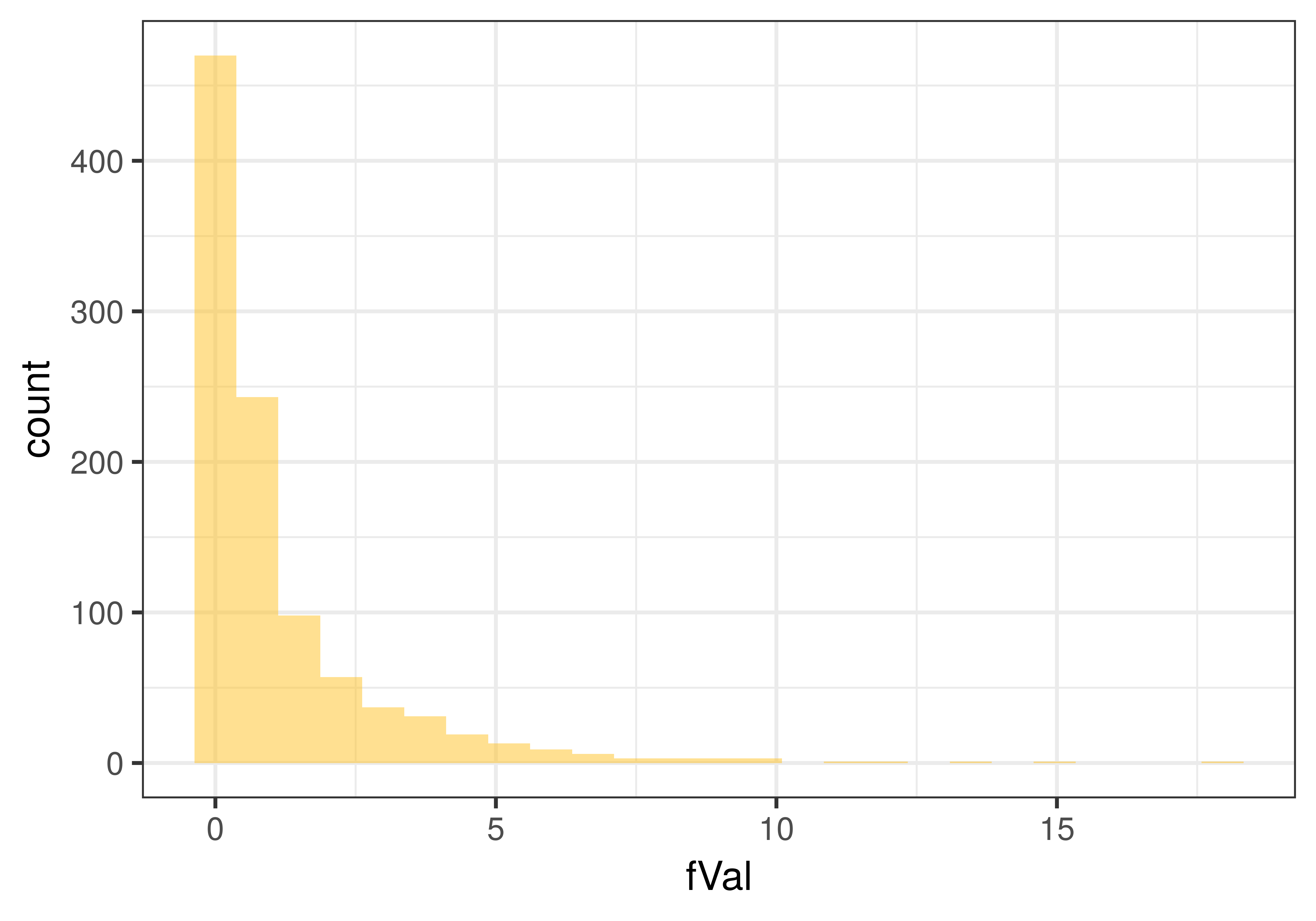
As you can see, the sampling distribution of F created based on the assumption that the empty model is true is still shaped like the F distribution, even though the model is a regression model and not a group model.
Use the code window and the tally() function to find out how many (or what proportion) of the 1000 Fs were greater than the sample F of 18.87.
require(coursekata)

# Simulate Check
set.seed(22)
x <- round(rnorm(1000, mean=15, sd=10), digits=1)
y <- x[x > 5 & x < 30]
TipPct <- sample(y, 44)
TipExperiment$Check <- (TipExperiment$Tip / TipPct) * 100
# we’ve saved the value 18.87 for you as sample_F
sample_F <- fVal(Tip ~ Check, data = TipExperiment)

# we have also generated 1000 Fs from the empty model of the DGP
sdoF <- do(1000) * fVal(shuffle(Tip) ~ Check, data = TipExperiment)

# how many fVals are larger than sample_F?
tally()
# we’ve saved the value 18.87 for you as sample_F
sample_F <- fVal(Tip ~ Check, data = TipExperiment)

# we have also generated 1000 Fs from the empty model of the DGP
sdoF <- do(1000) * fVal(shuffle(Tip) ~ Check, data = TipExperiment)

# how many fVals are larger than sample_F?
tally(~ fVal > sample_F, data = sdoF)
ex() %>% check_or(
    check_function(., "tally") %>% {
        check_arg(., "x") %>% check_equal()
        check_arg(., "data") %>% check_equal()
    },
    override_solution_code(., '{tally(~(fVal > sample_F), data= sdoF)}') %>%
        check_function(., "tally") %>% {
        check_arg(., "x") %>% check_equal()
        check_arg(., "data") %>% check_equal()
    }
)fVal > sample_F
TRUE FALSE
0 1000Although it is not impossible, not one of the 1000 randomized Fs (in our shuffled distribution; yours might be a little different) were as large as our sample F of 18.87. Based on this, we would estimate the p-value to be very small. And indeed, it is when we check our ANOVA table for the regression model (reproduced below), which reports a very small p-value of .0001 based on the mathematical F distribution.
supernova(lm(Tip ~ Check, data = TipExperiment))Analysis of Variance Table (Type III SS)
Model: Tip ~ Check
SS df MS F PRE p
----- --------------- | -------- -- -------- ------ ------ -----
Model (error reduced) | 1708.140 1 1708.140 18.865 0.3100 .0001
Error (from model) | 3802.837 42 90.544
----- --------------- | -------- -- -------- ------ ------ -----
Total (empty model) | 5510.977 43 128.162 Notice that the p-value is very small, .0001. If you think about what this number means, it means that 1 out of 10000 Fs (1/10000 = .0001) would be greater than our sample F. If we simulated 10000 Fs, one of them might be greater than our sample F. But it would be very rare. It is unlikely to get an F that large if the empty model is true. Based on this we would reject the empty model (null hypothesis).
Does Check Cause an Increase in Tip?
There appears to be a strong relationship between the size of the check and the amount that a table tips. And the fact that there is a very low p-value of .0001 indicates that a relationship this strong would be highly unlikely to have appeared in the data if the empty model were true. But should the low p-value give us confidence that size of the check actually caused the increase in Tip?
Causality cannot be inferred purely based on the results of statistical analysis; we must also take into account the research design.
When we were investigating the effect of smiley face on Tip we had the advantage of random assignment: each table at the restaurant was randomly assigned to Condition, to either get a smiley face or not. Because of random assignment, any variation in tips across conditions could be assumed to be either the result of smiley face (the one thing the researchers varied across conditions) or the result of pure randomness. A low p-value in this case would have supported the inference that smiley face caused higher tips because it gave us a basis for ruling out pure randomness as an explanation.
The analysis of the relationship between Check and Tip is a different story, however, because tables were not randomly assigned to check amounts. Because of this correlational design, we must consider the possibility that other factors, not measured by the researchers, might have actually caused the apparent relationship between Check and Tip. For example, if the tables with large checks were all celebrating something and those with smaller checks were not, we would have to consider that it might be the celebratory mood of the table, and not the check amount, that was causing the variation in tips.
Even in a correlational design, a low p-value can still help us rule out pure randomness as the only cause of variation in tip. But it cannot tell us that the variable Check is therefore a cause of variation in Tip. The variation could be due to check size, but also could be due to other confounding variables that we haven’t measured or even considered. In a correlational research design, p-value does not necessarily indicate a causal relationship.