13.7 Deciding Which Predictors to Include in a Model
From the analyses above, it is clear that a model including both Neighborhood and HomeSizeK is better, not only than the empty model, but than a model that includes only one of these predictors. But it’s not always true that two predictors are better than one. Deciding which variables to include in a model is an art and requires judgment.
Let’s look at another model for predicting PriceK in the Smallville data set. But this time let’s use HomeSizeK and HasFireplace as the two predictor variables. Below we’ve printed out the ANOVA table for this new multivariate model.
supernova(lm(PriceK~ HasFireplace + HomeSizeK, data = Smallville))Analysis of Variance Table (Type III SS)
Model: PriceK ~ HasFireplace + HomeSizeK
SS df MS F PRE p
------------ --------------- | ---------- -- --------- ------ ------ -----
Model (error reduced) | 103083.491 2 51541.745 11.854 0.4498 .0002
HasFireplace | 6438.722 1 6438.722 1.481 0.0486 .2335
HomeSizeK | 14673.576 1 14673.576 3.375 0.1042 .0765
Error (from model) | 126094.002 29 4348.069
------------ --------------- | ---------- -- --------- ------ ------ -----
Total (empty model) | 229177.493 31 7392.822The p-value on the Model (error reduced) row tells us that the multivariate model of the DGP is preferable to the empty model. Indeed, we can see from the overall PRE that the multivariate model accounts for a whopping 0.44 of the variation in PriceK, which is substantial.
The PREs for each of the predictor variables, however, present us with a puzzle. While the two-predictor model explains 44% of the variation in price, HomeSizeK explains only about 10% of the variation, and HasFireplace, 5%. Furthermore, the p-values for neither HomeSizeK nor HasFireplace fall below our .05 criterion, meaning that we can’t rule out that either of these effects might just be the result of random sampling variation from a DGP in which both effects are equal to 0. How is it possible that the individual variables explain so little compared with the overall model?
PriceK ~ HomeSizeK + Neighborhood
|
PriceK ~ HomeSizeK + HasFireplace
|
|---|---|
|

|
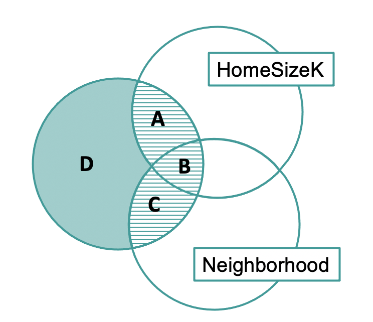
The PREs for HomeSizeK (region A) and HasFireplace (region C) tell us about each variable’s unique contribution. The unique contributions are small, but region B, which represents the overlapping contributions of the two variables is large. This is why the overall model has a much larger PRE than the individual predictors.
Even though these Venn diagrams are not exactly to scale, we can use them to reason about the relationships between the predictor and outcome variables. Based on this Venn diagram, specifically because of the large overlap, we might suspect that HomeSizeK and HasFireplace are highly related to one another.
Comparing the Multivariate and Single-Predictor Models
We’ve put some code in the window below to produce (again) the supernova table for the multivariate model (PriceK ~ HomeSizeK + HasFireplace). Add some code to get two more tables, one for the single-predictor model using HomeSizeK, the other for the single-predictor model using HasFireplace.
require(coursekata)

# delete when coursekata-r updated
Smallville <- read.csv("https://docs.google.com/spreadsheets/d/e/2PACX-1vTUey0jLO87REoQRRGJeG43iN1lkds_lmcnke1fuvS7BTb62jLucJ4WeIt7RW4mfRpk8n5iYvNmgf5l/pub?gid=1024959265&single=true&output=csv")
Smallville$Neighborhood <- factor(Smallville$Neighborhood)
Smallville$HasFireplace <- factor(Smallville$HasFireplace)
# code to make ANOVA table for multivariate model
supernova(lm(PriceK ~ HomeSizeK + HasFireplace, data = Smallville))

# add code to get ANOVA tables for each of the two single-predictor models
supernova(lm(PriceK~ HomeSizeK + HasFireplace, data = Smallville))
supernova(lm(PriceK~ HasFireplace, data = Smallville))
supernova(lm(PriceK~ HomeSizeK, data = Smallville))
# temporary SCT
ex() %>% check_error()
Model: PriceK ~ HasFireplace + HomeSizeK

                                        SS df        MS      F    PRE     p
 ------------ --------------- | ---------- -- --------- ------ ------ -----
        Model (error reduced) | 103083.491  2 51541.745 11.854 0.4498 .0002
 HasFireplace                 |   6438.722  1  6438.722  1.481 0.0486 .2335
    HomeSizeK                 |  14673.576  1 14673.576  3.375 0.1042 .0765
        Error (from model)    | 126094.002 29  4348.069
 ------------ --------------- | ---------- -- --------- ------ ------ -----
        Total (empty model)   | 229177.493 31  7392.822
 Model: PriceK ~ HasFireplace

                                 SS df        MS      F    PRE     p
 ----- --------------- | ---------- -- --------- ------ ------ -----
 Model (error reduced) |  88409.915  1 88409.915 18.842 0.3858 .0001
 Error (from model)    | 140767.578 30  4692.253
 ----- --------------- | ---------- -- --------- ------ ------ -----
 Total (empty model)   | 229177.493 31  7392.822
 Model: PriceK ~ HomeSizeK

                                 SS df        MS      F    PRE     p
 ----- --------------- | ---------- -- --------- ------ ------ -----
 Model (error reduced) |  96644.769  1 96644.769 21.876 0.4217 .0001
 Error (from model)    | 132532.724 30  4417.757
 ----- --------------- | ---------- -- --------- ------ ------ -----
 Total (empty model)   | 229177.493 31  7392.822
Take some time to compare the three ANOVA tables you produced. There are a few different things to notice about these ANOVA tables; we will discuss some of these below.
In the table below we have pulled out the PREs for HasFireplace and HomeSizeK for the three models. Consistent with what was represented in the Venn diagram, the PRE for HasFireplace went from 0.0486 to 0.3858 when we dropped HomeSizeK out of the model. Similarly, the PRE for HomeSizeK went from 0.1042 to 0.4217 when we dropped HasFireplace from the model. Both of the single-predictor models have very low p-values (0.0001).
| Model |
PRE for HasFireplace
|
PRE for HomeSizeK
|
|---|---|---|
PriceK ~ HasFirePlace + HomeSizeK
|
.0486 | .1042 |
PriceK ~ HasFirePlace
|
.3858 | — |
PriceK ~ HomeSizeK
|
— | .4217 |
The reason for this result is the overlap represented in the Venn diagram by region B, something statisticians call redundancy or multicollinearity. You can confirm that HomeSizeK and HasFireplace have a lot of redundancy, or shared variance, by plotting PriceK by HomeSizeK and using color to highlight those homes with fireplaces.

The redundancy between the two predictors is visible in the graph: homes with fireplaces tend to be larger than homes without; and larger homes are more likely to be the ones that have fireplaces.
In cases of high multicollinearity between two predictors – such as we have between HomeSizeK and HasFireplace – we need to see how much PRE we gain by including both predictors in the model. In this case, we don’t gain much: the PRE for the HomeSizeK model is .42, but for the multivariate model it only increases to .45. We might prefer to just stick with the HomeSizeK model.
We always want to keep in mind the tradeoff between reduction in error and the added complexity of having both predictor variables in the model. Is the multivariate model a good deal?
If we go back to the ANOVA tables we can see that the F statistic for the multivariate model is 11.85, whereas for the HomeSizeK model it is a whopping 21.88! This is a sign that we are reducing error a lot more per parameter estimated in the HomeSizeK model than in the multivariate model. We would probably just use the HomeSizeK model for now.
Considering Causality in Multivariate Models
Another reason to prefer the single-predictor HomeSizeK model has to do with causality. What is really causing a house to be more expensive? Is it the fireplace, or is it the additional square feet? If all we care about is prediction, it wouldn’t matter which model we chose. But often we are trying to find out what the causes of variation are.
Both would have some effect. But probably the square footage would have a bigger impact than the fireplace. The single-predictor HomeSizeK model does a good job predicting, uses only one degree of freedom, and represents our understanding of what causes variation in home prices.