10.8 Pairwise Comparisons
It might be good enough just to know that the complex model, the one that includes game, is significantly better than the empty model. But sometimes we want to know more than that. We want to know which of the three games, specifically, are more effective in the DGP, and which just appear more effective because of sampling variation.
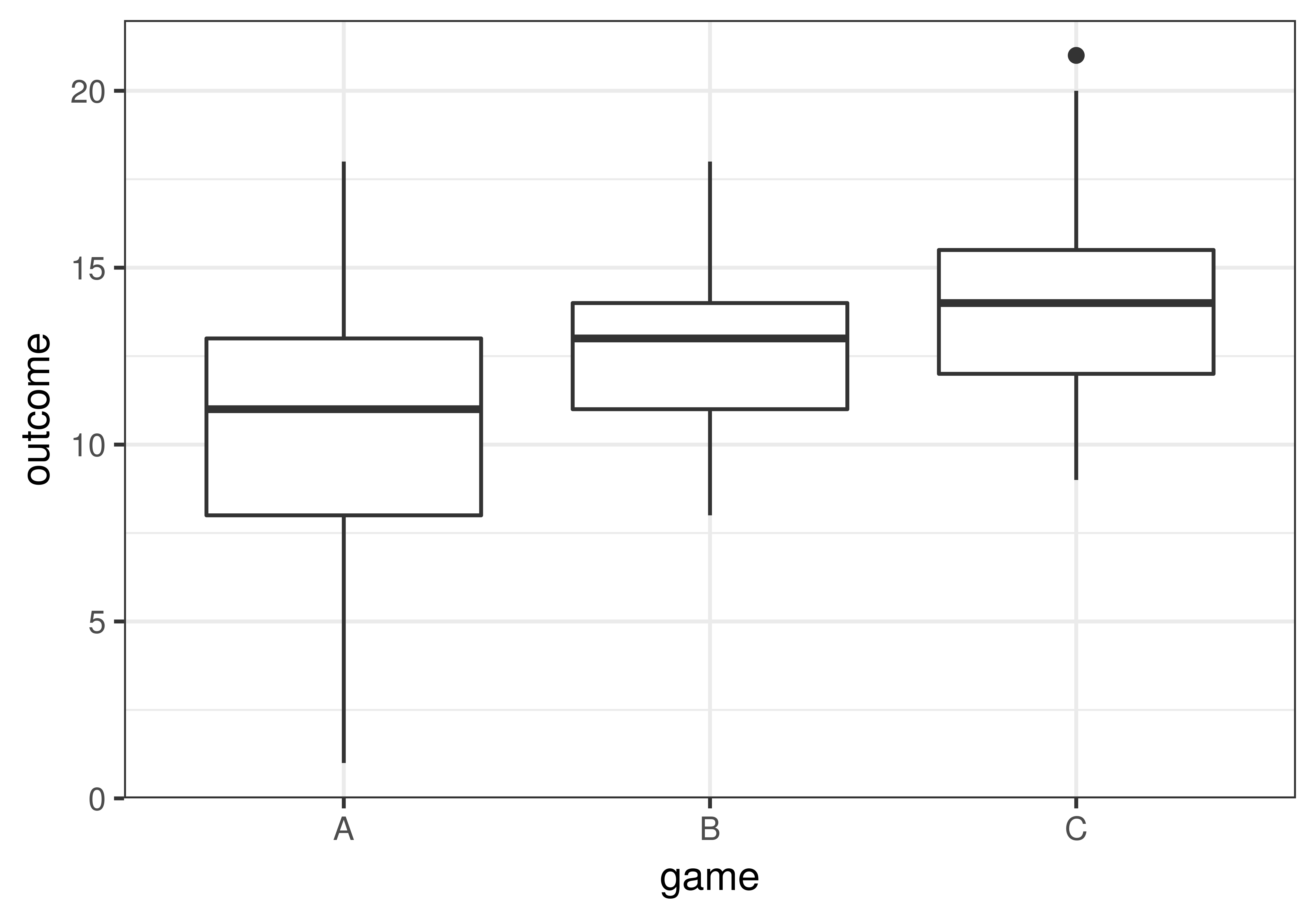
In our data (we’ve reproduced the boxplot below), it appears that game C’s students learned more than game B’s, who in turn learned more than game A’s. But such differences could be caused by sampling variation and not by real differences in the DGP. If we were to claim there is a difference in the DGP but it was actually just a difference caused by sampling variation, we would be fooled by chance (i.e., making a Type I Error).
To figure out which groups differ from each other in the DGP we can do three model comparisons, each designed to test the difference between one of the possible pairs of the three games: A vs. B, B vs. C, and A vs. C. The three model comparisons would be:
- a model in which A and B differ to one in which they are the same (the empty model);
- a model in which B and C differ compared to the empty model; and
- a model in which A and C differ compared with the empty model.
The models being compared for all three pairwise comparisons would be represented the same way in GLM notation:
Model comparing two games: \(Y_i=\beta_0+\beta_1X_i+\epsilon_i\)
Versus the empty model: \(Y_i=\beta_0+\epsilon_i\)
In other words, we would be doing three separate two-group comparisons, where \(X_i\) is coded 0 or 1 depending on which of the two games are being compared. Each comparison would yield a separate F statistic, which we could interpret using the appropriate F-distribution.
The pairwise() Function
A handy way to implement these pairwise model comparisons is using the pairwise() function in the supernova R package. Previously, we saved the three-group model of game predicting outcome in an R object called game_model. We can run the code below to get the pairwise comparisons.
pairwise(game_model, correction="none")The pairwise() function produces this output:
Model: outcome ~ game

Levels: 3

Family-wise error-rate: 0.143


  group_1 group_2  diff pooled_se     t    df lower upper p_val
  <chr>   <chr>   <dbl>     <dbl> <dbl> <int> <dbl> <dbl> <dbl>
1 B       A       2.086     0.516 4.041   102 1.229 2.942 .0001
2 C       A       3.629     0.516 7.031   102 2.772 4.485 .0000
3 C       B       1.543     0.516 2.990   102 0.686 2.400 .0035
Notice that in the pairwise table, there is a column called p_val at the end. This is the same p-value that we have been learning about: the probability of generating a statistic (in this case \(b_1\), the mean difference) more extreme than our sample if the empty model is true.
According to these individual pairwise comparisons, it seems as though all three groups are different from each other! But now that we are doing 3 “tests” of significance instead of just one overall F test of the three-group model, we have created a new problem: the problem of simultaneous inference.
The Problem of Simultaneous Comparisons
The problem of simultaneous inference is this: when we do an F test, we set an alpha level to define what will count as an “unlikely” sample F. The alpha indicates the amount of Type I error that we can tolerate. By setting alpha at .05 we are saying that if we get an F statistic with probability of less than .05 of coming from the empty model we are okay rejecting the empty model, even though there is a .05 chance of being wrong.
But look at this line that appears above the table in the output of pairwise():
Family-wise error-rate: 0.143What does this mean? We specified that we would be okay with a Type I error rate of .05, but this output suggests that we have an error rate of .14. That’s almost 3 times the Type I error rate we had set as our criterion.
If we set our Type I error rate at .05 (that is, we define .05 of the least likely F values as unlikely) and we do a lot of F tests, we will make a Type I error, on average, one out of every 20 times (that is, .05 of the time), rejecting the empty model when, in fact, the empty model is true. On the flipside, that means we avoid making a Type I error .95 of the time.
This is okay if all we care about is a single F test. But if we do three F tests simultaneously (as we do when we make pairwise comparisons of three groups), we want to achieve a .95 rate of avoiding Type I error across all three F tests, not just for each one separately.
You can think of it like flipping a coin. If you flip a coin once, the probability that it will come up heads is .50. But if you flip a coin three times, the probability of all three coming up heads is a lot less than .50. Similarly, if you do a single F test, the probability of avoiding a Type I error is .95. But if you do three F tests (e.g., three pairwise comparisons), the probability of avoiding a Type I error is a lot less than .95.
How much less than .95? If the probability of one test not being wrong is .95, the probability that none of the three tests is wrong would be \((.95*.95*.95)\), or 0.857. Therefore, the probability that any one of these three tests is wrong is 1 minus 0.857, or 0.143, which is what our output reported as the family-wise error rate. What this means is that the probability of making a Type I error on any one of the three comparisons is 0.143 (which is a lot higher than 0.05).
Adjusting the Family-Wise Error Rate
There are a number of ways to correct for the problem of simultaneous comparisons. The simplest is called the Bonferroni adjustment, named after the gentleman who proposed it. If we want to maintain a .95 chance of not making a Type I error on any of our comparisons, we would simply multiply the p-value of each test times the number of comparisons (in this case, 3) before comparing it to the alpha criterion.
The pairwise() function can make this correction by setting the argument correction = "Bonferroni".
pairwise(game_model, correction = "Bonferroni")The Bonferroni adjustment is straightforward, but some think it is overly conservative, in other words, that it’s trying too hard to protect us from making Type I error. The corrected p-value can get very large if the number of simultaneous comparisons gets large. Although this decreases the chance of making a Type I error, it increases the chance of making a Type II error, i.e., of not detecting a difference when one does exist.
Tukey’s Honestly Significant Difference Test
Another way to adjust the p-value is to use Tukey’s Honestly Significant Difference test, or Tukey’s HSD for short. This method tries to strike a more even balance between the two priorities: reducing the probability of Type I error and not overly inflating the probability of Type II error.
The procedure was invented by a man named John Tukey. Without getting into the details (which are more complex than for the Bonferroni adjustment), suffice it to say that in the Tukey HSD, like in the Bonferroni, p-values are adjusted upward to keep the family-wise error at a specified level (e.g., .05). Usually, though, the adjustment is not as extreme as it is using the Bonferroni method.
The pairwise() function we used above can be used to generate corrected p-values based on Tukey’s HSD. In fact, because this is a popular method, Tukey HSD-corrected p-values are the default:
pairwise(game_model)We could also add in the argument correction = "Tukey" to get Tukey adjusted p-values.
In the code window below, run pairwise() on the game_model twice, once with no correction ("none") and once with the Tukey correction. Compare the two outputs and notice what happens to the p-values.
require(coursekata)

# import game_data
students_per_game <- 35
game_data <- data.frame(
    outcome = c(16,8,9,9,7,14,5,7,11,15,11,9,13,14,11,11,12,14,11,6,13,13,9,12,8,6,15,10,10,8,7,1,16,18,8,11,13,9,8,14,11,9,13,10,18,12,12,13,16,16,13,13,9,14,16,12,16,11,10,16,14,13,14,15,12,14,8,12,10,13,17,20,14,13,15,17,14,15,14,12,13,12,17,12,12,9,11,19,10,15,14,10,10,21,13,13,13,13,17,14,14,14,16,12,19),
    game = c(rep("A", students_per_game), rep("B", students_per_game), rep("C", students_per_game))
)
# this code fits the game model and saves it as game_model
game_model <- lm(outcome ~ game, data = game_data)

# Run pairwise comparisons with no corrections
pairwise( )

# Run pairwise comparisons with Tukey corrections
pairwise( )
# this code fits the game model and saves it as game_model
game_model <- lm(outcome ~ game, data = game_data)

# modify this code to generate pairwise plots
pairwise(game_model, correction = "none")

# Run pairwise comparisons with Tukey corrections
pairwise(game_model)
ex() %>% {
       check_function(., "pairwise", index = 1) %>%
           check_result() %>%
           check_equal()

       check_function(., "pairwise", index = 2) %>%
           check_result() %>%
           check_equal()
}── Pairwise t-tests ────────────────────────────────────────────────────────────
Model: outcome ~ game
Levels: 3
Family-wise error-rate: 0.143
group_1 group_2 diff pooled_se t df lower upper p_val
<chr> <chr> <dbl> <dbl> <dbl> <int> <dbl> <dbl> <dbl>
1 B A 2.086 0.516 4.041 102 1.229 2.942 .0001
2 C A 3.629 0.516 7.031 102 2.772 4.485 .0000
3 C B 1.543 0.516 2.990 102 0.686 2.400 .0035── Tukey's Honestly Significant Differences ────────────────────────────────────
Model: outcome ~ game
Levels: 3
Family-wise error-rate: 0.05
group_1 group_2 diff pooled_se q df lower upper p_adj
<chr> <chr> <dbl> <dbl> <dbl> <int> <dbl> <dbl> <dbl>
1 B A 2.086 0.516 4.041 102 0.350 3.822 .0142
2 C A 3.629 0.516 7.031 102 1.893 5.364 .0000
3 C B 1.543 0.516 2.990 102 -0.193 3.279 .0920In the Tukey pairwise comparisons, the p-values were adjusted up in order to maintain a family-wise error rate of 0.05.
Take a closer look at the comparison of games B and C in the unadjusted output.
  group_1 group_2  diff pooled_se     t    df lower upper p_val
3 C       B       1.543     0.516 2.990   102 0.686 2.400 .0035
This comparison was considered “unlikely to have been generated by the empty model” (e.g., lower than .05). The unadjusted comparison would conclude that games B and C were significantly different. But after the Tukey adjustment (shown below), the p-value is not lower than .05. Thus, games B and C are not significantly different.
  group_1 group_2  diff pooled_se     t    df  lower upper p_val
3 C       B       1.543     0.516 2.990   102 -0.193 3.279 .0920